This function generates plots for all components of a drift diffusion model (DDM), such as drift rate, boundary, and starting condition. Each component is plotted against the time or evidence space, allowing for visual inspection of the model's behavior across different conditions.
Usage
# S3 method for class 'drift_dm'
plot(x, ..., conds = NULL, col = NULL, xlim = NULL, bundle_plots = TRUE)
Arguments
- x
an object of class drift_dm
- ...
additional graphical arguments passed to plotting functions. See
set_default_arguments()for the full list of supported options.- conds
a character vector specifying the conditions to plot. Defaults to all available conditions.
- col
a character vector specifying colors for each condition. If a single color is provided, it is repeated for all conditions.
- xlim
a numeric vector of length 2, specifying the x-axis limits.
- bundle_plots
logical, indicating whether to display separate panels in a single plot layout (
FALSE), or to plot them separately (TRUE).
Details
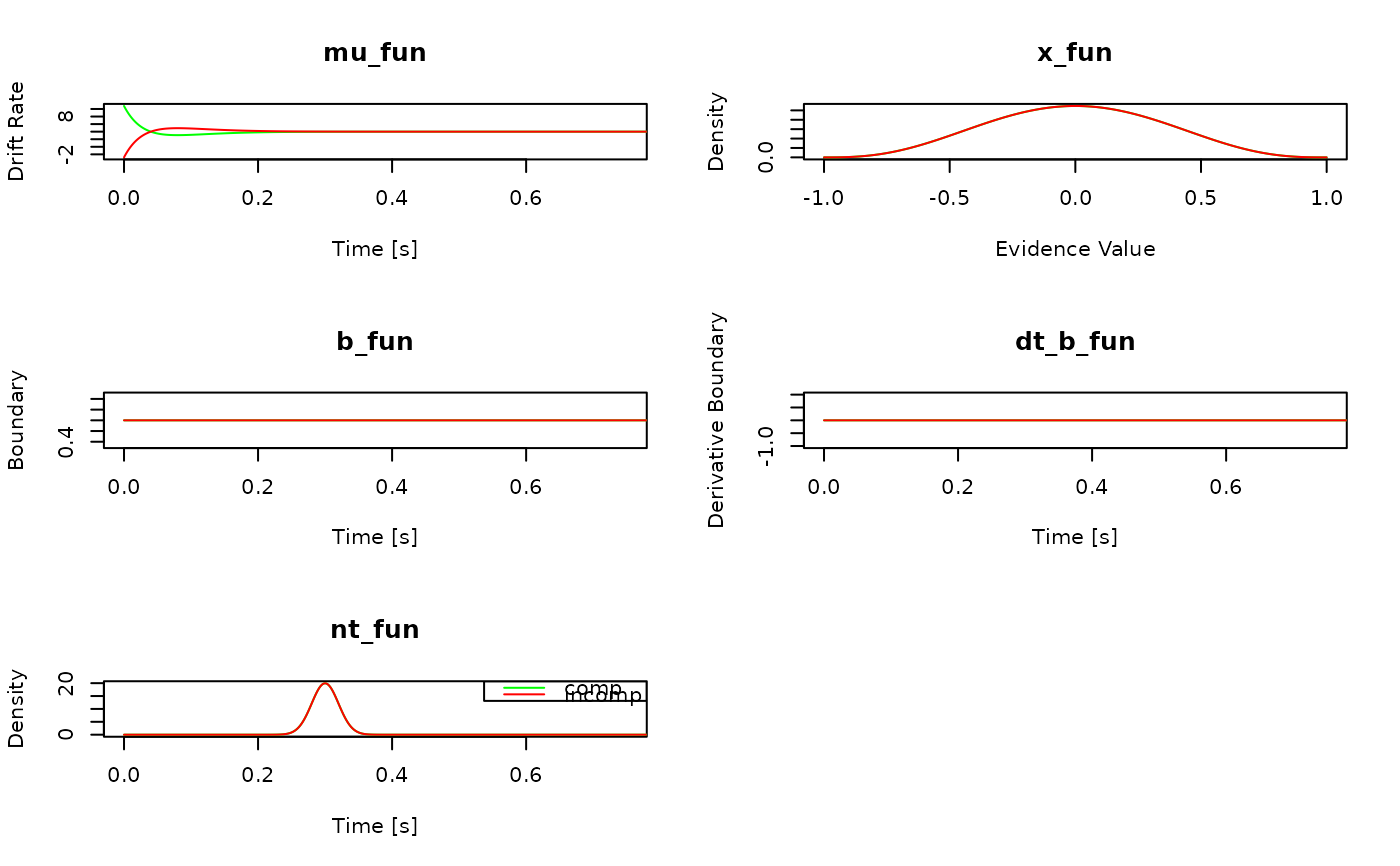
The plot.drift_dm function provides an overview of key DDM components,
which include:
mu_fun: Drift rate over time.mu_int_fun: Integrated drift rate over time (if required by the specifiedsolverof the model).x_fun: Starting condition as a density across evidence values.b_fun: Boundary values over time.dt_b_fun: Derivative of the boundary function over time.nt_fun: Non-decision time as a density over time.
Examples
# plot the component functions of the Ratcliff DDM
plot(ratcliff_dm())
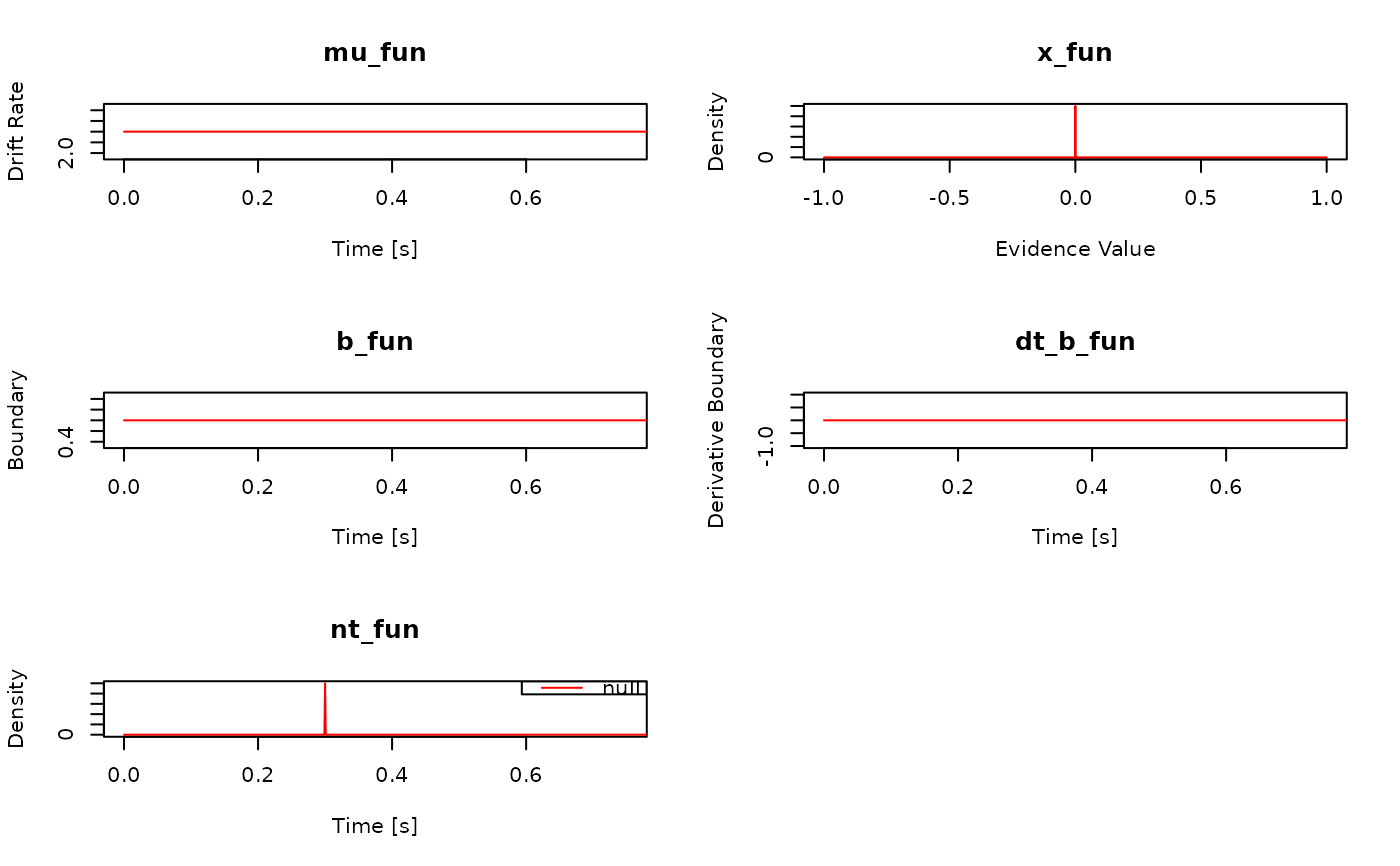 plot(ratcliff_dm(var_non_dec = TRUE))
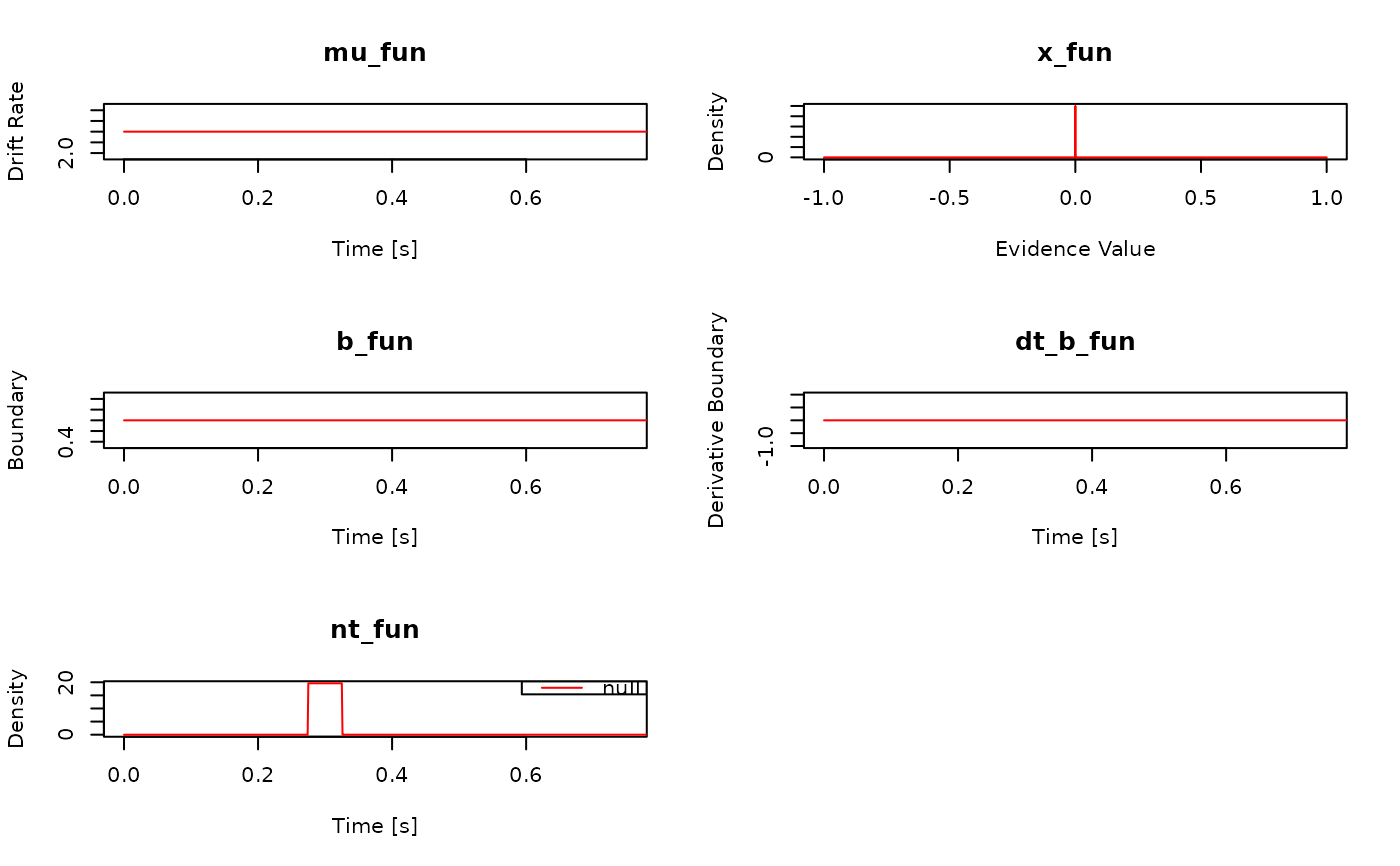 # Note: the variability in the drift rate for the Ratcliff DDM
# is not plotted! This is because it is not actually stored as a component
# function.
# plot the component functions of the DMC model
plot(dmc_dm(), col = c("green", "red"))
# Note: the variability in the drift rate for the Ratcliff DDM
# is not plotted! This is because it is not actually stored as a component
# function.
# plot the component functions of the DMC model
plot(dmc_dm(), col = c("green", "red"))