The dRiftDM package provides pre-built Drift-Diffusion
Models (DDMs; see vignette("dRiftDM", "dRiftDM")). However,
one of the strengths of dRiftDM is that it allows you to
customize models by specifying arbitrary component functions for the
drift rate, boundary, etc., and how the parameters relate across
conditions.
The Model Structure in dRiftDM
To better understand how we can customize a DDM, we first need to
understand how models are structured within dRiftDM and how
model predictions are derived. Each model in dRiftDM is
essentially a list that has (among other things) two important
entries:
flex_prms_objcontaining a so-calledflex_prmsobject, which controls the parameterscomp_funsa list of “component” functions that represent the model’s drift rate, boundary, etc.
We can see these entries by addressing the labels of the underlying list:
a_model <- ratcliff_dm() # some model
names(a_model) # the entries of the underlying list
#> [1] "flex_prms_obj" "prms_solve"    "solver"        "comp_funs"
#> [5] "cost_function"
With the flex_prms object (stored as the first entry),
we can specify the parameters of the model and also control how each
parameter relates across conditions. For example, we could specify that
a parameter A in condition incomp is the
negative of parameter A in condition comp. Or
we could specify that a parameter muc is estimated
separately for two conditions.
With the functions stored in comp_funs (the fourth
entry), we can control the drift rate, boundary, starting point, and
non-decision time. Each function takes a set of arguments, including the
model parameters, and returns a vector of values. For example, the drift
rate function returns the drift rate of the diffusion model for each
time step.
When deriving the model predictions, the comp_funs are
evaluated with the currently set parameter values controlled by the
flex_prms object. Dedicated numerical algorithms in the
depths of dRiftDM then derive the model’s predicted
probability density functions of response times, separately for each
possible response choice. It is important to emphasize this interaction
of comp_funs with the flex_prms object, as you
will need to ensure that the two work together smoothly. For example, a
function stored in comp_funs might fail if it is given a
parameter vector that it does not expect. Or a model might not work as
expected if a function stored in comp_funs doesn’t consider
a certain parameter. The workflow is emphasized in the following
diagram:

Given this, there are two ways to customize a model, and depending on the problem, you may need to consider both or only one.
1.) You can modify a model’s flex_prms object. This is
relevant whenever you want to change how the parameters of a model
relate across conditions.
2.) You can customize the component functions. This is relevant whenever you want to have a different drift rate, boundary, starting point, or non-decision time.
Modifying flex_prms objects
We can access the underlying flex_prms object of a model
with the generic flex_prms() accessor method:
# Create a model (here the Diffusion Model for Conflict Tasks, DMC)
ddm <- dmc_dm()
flex_prms(ddm)
#> Parameter Values:
#>        muc   b non_dec sd_non_dec  tau a    A alpha
#> comp     4 0.6     0.3       0.02 0.04 2  0.1     4
#> incomp   4 0.6     0.3       0.02 0.04 2 -0.1     4
#>
#> Parameter Settings:
#>        muc b non_dec sd_non_dec tau a A alpha
#> comp   1   2 3       4          5   0 6 7
#> incomp 1   2 3       4          5   0 d 7
#>
#> Special Dependencies:
#> A ~ incomp == -(A ~ comp)
#>
#> Custom Parameters:
#>        peak_l
#> comp     0.04
#> incomp   0.04
Here we see the two core aspects of any flex_prms object
(see also the first print statement in
vignette("dRiftDM", "dRiftDM") for more information):
The Parameter Values shows you the current parameter values for all conditions.
The Parameter Settings show how each parameter behaves across conditions.
Modifying How Each Parameter Behaves Across Conditions
The Parameter Settings are relevant to model
customization, and we can change them with the
modify_flex_prms() method. The function takes a model and a
set of instructions as a string. For example, if we
want muc to vary freely across conditions, we can write
ddm_free_muc <- modify_flex_prms(
  ddm, # the model
  instr = "muc ~" # an instructions in a formula-like format
)
flex_prms(ddm_free_muc)
#> Parameter Values:
#>        muc   b non_dec sd_non_dec  tau a    A alpha
#> comp     4 0.6     0.3       0.02 0.04 2  0.1     4
#> incomp   4 0.6     0.3       0.02 0.04 2 -0.1     4
#>
#> Parameter Settings:
#>        muc b non_dec sd_non_dec tau a A alpha
#> comp   1   3 4       5          6   0 7 8
#> incomp 2   3 4       5          6   0 d 8
#>
#> Special Dependencies:
#> A ~ incomp == -(A ~ comp)
#>
#> Custom Parameters:
#>        peak_l
#> comp     0.04
#> incomp   0.04
Since there are now two numbers for muc under
Parameter Settings, this parameter can take different
values for different conditions. This is also why coef()
now provides two (modifiable) values for muc per
condition:
coef(ddm) # in this model muc is the same for all conditions
#>        muc          b    non_dec sd_non_dec        tau          A      alpha
#>       4.00       0.60       0.30       0.02       0.04       0.10       4.00

coef(ddm_free_muc) # here muc can be different for the conditions
#>   muc.comp muc.incomp          b    non_dec sd_non_dec        tau          A
#>       4.00       4.00       0.60       0.30       0.02       0.04       0.10
#>      alpha
#>       4.00

coef(ddm_free_muc)[1] <- 5
coef(ddm_free_muc)
#>   muc.comp muc.incomp          b    non_dec sd_non_dec        tau          A
#>       5.00       4.00       0.60       0.30       0.02       0.04       0.10
#>      alpha
#>       4.00
modify_flex_prms() supports the following instructions
(see the documentation for the syntax of each instruction):
The vary instruction: Allows parameters to be estimated independently across conditions.
The “restrain” instruction: Forces parameters to be identical across conditions.
The “fix” instruction: Keeps parameters constant. They don’t vary while the remaining parameters are estimated.
The “special dependency” instruction: Sometimes we want a parameter in one condition to depend on another parameter in a second condition. An example of this is already shown in the
flex_prms(ddm)output above. Here the parameterAin the conditionincompis the negative of the parameter in the conditioncomp.The “custom parameter” instruction: Sometimes, we want to calculate a linear combination of the model parameters. An example for this is already shown in the
flex_prms(ddm)output above. Here, we have the custom parameterpeak_l(for “peak latency”), which ispeak_l = (a-1)*tau(the equation is not apparent from the output).
Defining New Conditions
The current conditions of a model can be accessed with the
conds() method:
conds(ddm)
#> [1] "comp"   "incomp"
We can assign new values to change these conditions. For example, a researcher may want to introduce a neutral condition:
Here we receive a message reminding us that all parameter values have
been reset. In fact, when we print out the underlying
flex_prms object, we see that the previous settings are
gone (e.g., A in the incomp condition is no
longer the negative of A in the comp
condition):
flex_prms(ddm)
#> Parameter Values:
#>         muc   b non_dec sd_non_dec  tau a   A alpha
#> comp      4 0.6     0.3       0.02 0.04 2 0.1     4
#> neutral   4 0.6     0.3       0.02 0.04 2 0.1     4
#> incomp    4 0.6     0.3       0.02 0.04 2 0.1     4
#>
#> Parameter Settings:
#>         muc b non_dec sd_non_dec tau a A alpha
#> comp      1 2       3          4   5 6 7     8
#> neutral   1 2       3          4   5 6 7     8
#> incomp    1 2       3          4   5 6 7     8
While this may be a bit annoying in some cases, it actually makes
sense because there is no way for dRiftDM to know how the new conditions
relate to the old ones. Consequently, we now have to modify the
underlying flex_prms object again to suit our needs. For
example, we could restore the previous behavior for A in
the incomp condition, while setting A to zero
for the new neutral condition. We might also want to keep
a again fixed for all conditions:
instructions <- "
a <!>                      # 'a' is fixed across all conditions
A ~ incomp == -(A ~ comp)  # A in incomp is -A in comp
A <!> neutral              # A is fixed for the neutral condition
A ~ neutral => 0           # A is zero for the neutral condition
"

ddm <- modify_flex_prms(
  object = ddm,
  instr = instructions
)
print(ddm)
#> Class(es) dmc_dm, drift_dm
#> (model has not been estimated yet)
#>
#> Parameter Values:
#>         muc   b non_dec sd_non_dec  tau a    A alpha
#> comp      4 0.6     0.3       0.02 0.04 2  0.1     4
#> neutral   4 0.6     0.3       0.02 0.04 2  0.0     4
#> incomp    4 0.6     0.3       0.02 0.04 2 -0.1     4
#>
#> Parameter Settings:
#>         muc b non_dec sd_non_dec tau a A alpha
#> comp    1   2 3       4          5   0 6 7
#> neutral 1   2 3       4          5   0 0 7
#> incomp  1   2 3       4          5   0 d 7
#>
#> Special Dependencies:
#> A ~ incomp == -(A ~ comp)
#>
#> Deriving PDFS:
#>   solver: kfe
#>   values: sigma=1, t_max=3, dt=0.0075, dx=0.02, nt=400, nx=100
#>
#> Cost Function: neg_log_like
#>
#> Observed Data: NULL
Customizing Component Functions
As mentioned above, another way to customize a model is to change the
component functions for the drift rate, boundary, start point, or
non-decision time. We can access each component function using the
comp_funs() method:
ddm <- dmc_dm() # some pre-built model
names(comp_funs(ddm))
#> [1] "mu_fun"     "mu_int_fun" "x_fun"      "b_fun"      "dt_b_fun"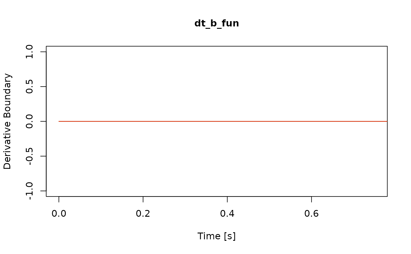
#> [6] "nt_fun"mu_fun()andmu_int_fun()return the drift rate and its integral. The integral is required as an entry, but is only evaluated if the user chooses the non-default method “im_zero” to derive model predictions.x_fun()returns the density for the initial distribution.The
b_fun()anddt_b_fun()functions returns the (upper) boundary and its derivative, respectively.Finally,
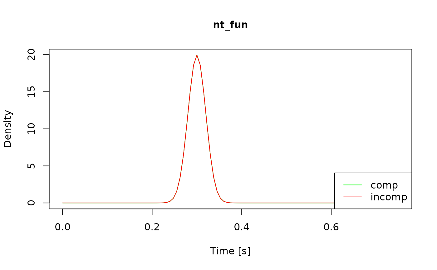
nt_fun()returns the density of the non-decision time.
A number of predefined component functions are already available via
component_shelf() (see the documentation for a description
of each function):
all_funs <- component_shelf()
names(all_funs)
#>  [1] "mu_constant"         "mu_dmc"              "mu_ssp"
#>  [4] "mu_int_constant"     "mu_int_dmc"          "x_dirac_0"
#>  [7] "x_beta"              "x_uniform"           "b_constant"
#> [10] "b_hyperbol"          "b_weibull"           "dt_b_constant"
#> [13] "dt_b_hyperbol"       "dt_b_weibull"        "nt_constant"
#> [16] "nt_uniform"          "nt_truncated_normal" "dummy_t"
The structure of each of these component functions is generally the
same. The drift rate, boundary, and non-decision time functions (i.e.,
mu_fun, mu_int_fun, b_fun,
dt_b_fun, and nt_fun) must have the following
declaration:
... <- function(prms_model, prms_solve, t_vec, one_cond, ddm_opts) {
  ...
}-
prms_modelis a named numeric vector and is identical to a row of the Parameter Values stored within theflex_prmsobject of a model (see the first part of the following output).
flex_prms(ddm)
#> Parameter Values:
#>        muc   b non_dec sd_non_dec  tau a    A alpha
#> comp     4 0.6     0.3       0.02 0.04 2  0.1     4
#> incomp   4 0.6     0.3       0.02 0.04 2 -0.1     4
#>
#> Parameter Settings:
#>        muc b non_dec sd_non_dec tau a A alpha
#> comp   1   2 3       4          5   0 6 7
#> incomp 1   2 3       4          5   0 d 7
#>
#> Special Dependencies:
#> A ~ incomp == -(A ~ comp)
#>
#> Custom Parameters:
#>        peak_l
#> comp     0.04
#> incomp 0.04-
prms_solveis a named numeric vector, including the diffusion constant and the discretization settings. It is identical to:
prms_solve(ddm)
#>   sigma   t_max      dt      dx      nt      nx
#> 1.0e+00 3.0e+00 7.5e-03 2.0e-02 4.0e+02 1.0e+02-
t_vecis a numeric vector, representing the time space. It is constructed fromdtandt_max:
t_max <- prms_solve(ddm)["t_max"]
dt <- prms_solve(ddm)["dt"]
t_vec <- seq(0, t_max, dt)
head(t_vec)
#> [1] 0.0000 0.0075 0.0150 0.0225 0.0300 0.0375
tail(t_vec)
#> [1] 2.9625 2.9700 2.9775 2.9850 2.9925 3.0000one_condis the label of the current condition for which the model is being evaluated (i.e., a row name of the Parameter Values).ddm_optsis taken directly from the model. It is used as a backdoor to inject arbitraryRobjects (see the final comments below for an example)
Each drift rate, boundary, and non-decision time function must return
a numeric vector of the same length as t_vec (see below for
examples).
For the drift rate, these returned values represent the drift rate (or its integral) at each time step.
For the boundary (or its derivative), these values are the boundary values returned for the upper boundary at each time step. The lower boundary is always assumed to be the negative of the upper boundary. That is, the bounds are symmetric about zero.
Finally, the values returned for the non-decision time represent the density values of the respective distribution.
The declaration for the starting point function, x_fun,
is similar, with one exception. It must take the argument
x_vec:
... <- function(prms_model, prms_solve, x_vec, one_cond, ddm_opts) {
  ...
}-
x_vecis a numeric vector, with the (standardized) evidence space. It is constructed fromdxand spans from -1 to 1:
dx <- prms_solve(ddm)["dx"]
x_vec <- seq(-1, 1, dx)
Each starting point function must return a numeric vector of the same
length as x_vec, providing the density values of the
starting points over the evidence space.
In theory, you can simply replace component functions using the
replacement method for comp_funs(). However, at runtime,
the values for the arguments prms_model and
one_cond come from a row of the model’s parameter matrix
(i.e., from the underlying flex_prms object). Thus, you
must ensure that each component function can handle the values supplied.
Consequently, directly swapping functions only makes sense when the
model parameters remain the same. The more general approach is to write
a function that assembles the model.
The following sections provide examples for a custom …
- … drift rate (Example 1)
- … starting point (Example 2)
- … boundary (Example 3)
- … non-decision time (Example 4)
Example 1: Custom Drift Rate
Assume that we want a model with the following custom drift rate: Thus, in compatible conditions, the drift rate at each time step is the sum of the two drift rates and , while in incompatible conditions it is their difference.
First, we write the corresponding drift rate function like this:
cust_mu <- function(prms_model, prms_solve, t_vec, one_cond, ddm_opts) {
  # extract all parameters (one row of the parameter matrix)
  muc <- prms_model[["muc"]]
  mua <- prms_model[["mua"]]
  sign <- prms_model[["sign"]]

  # and return the drift rate at each time step
  mu <- rep(muc + sign * mua, length(t_vec))
  return(mu)
}
Within this function, we first extract the model parameters relevant
to the calculation of the drift rate. Then, depending on an auxiliary
parameter sign, we sum both parameters and return the
vector of drift rates for each time step.
The next step is to create a function that assembles the custom model
by calling dRiftDM’s backbone function drift_dm(). Here we
define vectors for all model parameters and conditions. We then assemble
the model using not only our custom drift rate function, but also
pre-built functions for the boundary, start point, and non-decision
time.1
Finally, we ensure that the auxiliary sign parameter works as intended
by modifying the parameter settings with
modify_flex_prms():
cust_model <- function() {
  # define all parameters and conditions
  prms_model <- c(
    muc = 3, # parameters for the custom drift rate function
    mua = 1,
    sign = 1,
    b = .6, # parameter for a time-independent boundary "b"
    non_dec = .2 # parameter for a non-decision time "non_dec"
  )
  conds <- c("comp", "incomp")

  # get access to pre-built component functions
  comps <- component_shelf()

  # call the drift_dm function which is the backbone of dRiftDM
  ddm <- drift_dm(
    prms_model = prms_model,
    conds = conds,
    subclass = "my_custom_model",
    mu_fun = cust_mu, # your custom drift rate function
    # of the drift rate is required per default
    x_fun = comps$x_dirac_0, # pre-built dirac delta on zero for the starting point
    b_fun = comps$b_constant, # pre-built time-independent boundary with parameter b
    dt_b_fun = comps$dt_b_constant, # pre-built derivative of the boundary
    nt_fun = comps$nt_constant # pre-built non-decision time with parameter non_dec
  )

  # modify the flex_prms object to achieve the desired behavior of 'sign'
  # -> don't consider 'sign' a free parameter to estimate and set it to -1
  # for incompatible conditions
  ddm <- modify_flex_prms(
    ddm,
    instr = "sign <!>
    sign ~ incomp => -1"
  )

  return(ddm)
}

ddm <- cust_model()
pdf_vals <- pdfs(ddm)
plot(pdf_vals$pdfs$comp$pdf_u)
If we want to use the “im_zero” method to derive model predictions
(see solver()), we also need to write a function for the
integral of the drift rate. Note, however, that the “im_zero” method is
primarily provided for backward compatibility, and it is usually not
needed; the default “kfe” method is recommended and often works fine.
Thus, especially novel users can just skip the following part.
cust_mu_int <- function(prms_model, prms_solve, t_vec, one_cond, ddm_opts) {
  # extract all parameters (one row of the parameter matrix)
  muc <- prms_model[["muc"]]
  mua <- prms_model[["mua"]]
  sign <- prms_model[["sign"]]

  # and return the integral of the drift rate
  mu <- (muc + sign * mua) * t_vec
  return(mu)
}
This function is then passed to the mu_int_fun argument
within the cust_model() function. Everything else is the
same.
Example 2: Custom Starting Point (Distribution)
Suppose we want a model where the starting point of the diffusion process is controlled by a parameter . If , the starting point is zero. If , the starting point is closer to the upper boundary. If , the start point is closer to the lower boundary. Such a custom starting point distribution might look like this:
cust_x <- function(prms_model, prms_solve, x_vec, one_cond, ddm_opts) {
  dx <- prms_solve[["dx"]]
  z <- prms_model[["z"]]
  stopifnot(z > 0, z < 1)

  # create a dirac delta for the starting point
  x <- numeric(length = length(x_vec))
  index <- round(z * (length(x) - 1)) + 1
  x[index] <- 1 / dx # make sure it integrates to 1
  return(x)
}
Then we write a function that assembles the custom model:
cust_model <- function() {
  # define all parameters and conditions
  prms_model <- c(
    z = .75, # parameter for the custom starting point
    muc = 4, # parameter for a time-independent drift rate "muc"
    b = .6, # parameter for a time-independent boundary "b"
    non_dec = .2 # parameter for a non-decision time "non_dec"
  )

  # each model must have a condition (in this example it is not relevant, so we just call it "foo")
  conds <- c("foo")

  # get access to pre-built component functions
  comps <- component_shelf()

  # call the drift_dm function which is the backbone of dRiftDM
  ddm <- drift_dm(
    prms_model = prms_model,
    conds = conds,
    subclass = "my_custom_model",
    mu_fun = comps$mu_constant, # time-independent drift rate with parameter muc
    mu_int_fun = comps$mu_int_constant, # respective integral of the drift rate
    x_fun = cust_x, # custom starting point function with parameter z
    b_fun = comps$b_constant, # time-independent boundary with parameter b
    dt_b_fun = comps$dt_b_constant, # respective derivative of the boundary
    nt_fun = comps$nt_constant # non-decision time with parameter non_dec
  )
  return(ddm)
}

ddm <- cust_model()
Example 3: Custom Boundary
Remark: This example shows a reimplementation of the already
pre-built b_hyperbol() and dt_b_hyperbol()
component functions (see component_shelf()). If you want a
model with a collapsing boundary, just jump to the
cust_model R chunk below and plug in the respective
pre-built component functions.
Suppose we want collapsing boundaries. The formula for the upper
boundary should be
where
is the initial value of the upper boundary,
is the rate of collapse, and
is the time at which the boundary has collapsed by half. Since
dRiftDM assumes symmetric boundaries, the lower bound is
.
The corresponding R function for this is:
# the boundary function
cust_b <- function(prms_model, prms_solve, t_vec, one_cond, ddm_opts) {
  b0 <- prms_model[["b0"]]
  kappa <- prms_model[["kappa"]]
  t05 <- prms_model[["t05"]]

  return(b0 * (1 - kappa * t_vec / (t_vec + t05)))
}
To make this work with dRiftDM, we also provide the
derivative of the boundary:
The corresponding R function for this is:
# the derivative of the boundary function
cust_dt_b <- function(prms_model, prms_solve, t_vec, one_cond, ddm_opts) {
  b0 <- prms_model[["b0"]]
  kappa <- prms_model[["kappa"]]
  t05 <- prms_model[["t05"]]

  return(-(b0 * kappa * t05) / (t_vec + t05)^2)
}
Then we write a function that assembles the custom model;
cust_model <- function() {
  # define all parameters and conditions
  prms_model <- c(
    b0 = .6, # parameters for the custom boundary
    kappa = .5,
    t05 = .15,
    muc = 4, # parameter for a time-independent drift rate "muc"
    non_dec = .2 # parameter for a non-decision time "non_dec"
  )

  # each model must have a condition
  # (in this example it is not relevant, so we just call it "foo")
  conds <- c("foo")

  # get access to pre-built component functions
  comps <- component_shelf()

  # call the drift_dm function which is the backbone of dRiftDM
  ddm <- drift_dm(
    prms_model = prms_model,
    conds = conds,
    subclass = "my_custom_model",
    mu_fun = comps$mu_constant, # time-independent drift rate with parameter muc
    mu_int_fun = comps$mu_int_constant, # respective integral of the drift rate
    x_fun = comps$x_dirac_0, # dirac delta on zero
    b_fun = cust_b, # custom time-dependent boundary
    dt_b_fun = cust_dt_b, # respective derivative of the boundary
    nt_fun = comps$nt_constant # non-decision time with parameter non_dec
  )
  return(ddm)
}
ddm <- cust_model()
Example 4: Custom Non-Decision Time
Remark: This example shows a reimplementation of the already
pre-built nt_uniform() component function (see
component_shelf().
Suppose we want a uniform non-decision time distribution with
parameters non_dec and range_non_dec:
cust_nt <- function(prms_model, prms_solve, t_vec, one_cond, ddm_opts) {
  # get the relevant parameters
  non_dec <- prms_model[["non_dec"]]
  range_non_dec <- prms_model[["range_non_dec"]]

  # get the settings for the time space discretization
  t_max <- prms_solve[["t_max"]]
  dt <- prms_solve[["dt"]]

  # calculate the density
  d_nt <- dunif(x = t_vec, min = non_dec - range_non_dec / 2, max = non_dec + range_non_dec / 2)
  d_nt <- d_nt / (sum(d_nt) * dt) # ensure it integrates to 1
  return(d_nt)
}
Then we write a function that assembles the custom model:
cust_model <- function() {
  # define all parameters and conditions
  prms_model <- c(
    non_dec = .2, # parameters for the custom non-decision time
    range_non_dec = .05,
    muc = 4, # parameter for a time-independent drift rate
    b = .6 # parameter for a time-independent boundary
  )

  # each model must have a condition
  # (in this example it is not relevant, so we just call it "foo")
  conds <- c("foo")

  # get access to pre-built component functions
  comps <- component_shelf()

  # call the drift_dm function which is the backbone of dRiftDM
  ddm <- drift_dm(
    prms_model = prms_model,
    conds = conds,
    subclass = "my_custom_model",
    mu_fun = comps$mu_constant, # time-independent drift rate with parameter muc
    mu_int_fun = comps$mu_int_constant, # respective integral of the drift rate
    x_fun = comps$x_dirac_0, # dirac delta on zero
    b_fun = comps$b_constant, # time-independent boundary b
    dt_b_fun = comps$dt_b_constant, # respective derivative of the boundary
    nt_fun = cust_nt # custom non-decision time
  )
  return(ddm)
}
ddm <- cust_model()
Final Comments
More Examples? The previous examples have shown you
how to tailor a model to your needs using custom component functions.
For more examples and inspiration, we suggest you take a look at the
source code of the predefined component functions. A list of all
component functions can be found in the documentation for
component_shelf().
?component_shelfThe source code for each function is available on our Github page here. Alternatively, you can access the source code from R like this:
all_funs <- component_shelf() # all functions
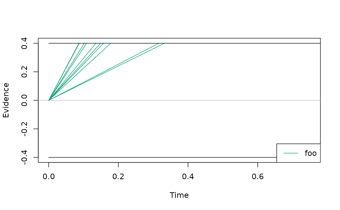
View(all_funs$x_uniform) # see the code for x_uniformHow do I check that the model is working as intended? There are three ways to perform sanity checks. First, to check the boundary and drift rate, you can plot the expected time course of your diffusion model:
ddm <- dmc_dm()
test <- simulate_traces(ddm, k = 1, sigma = 0, add_x = FALSE)
plot(test)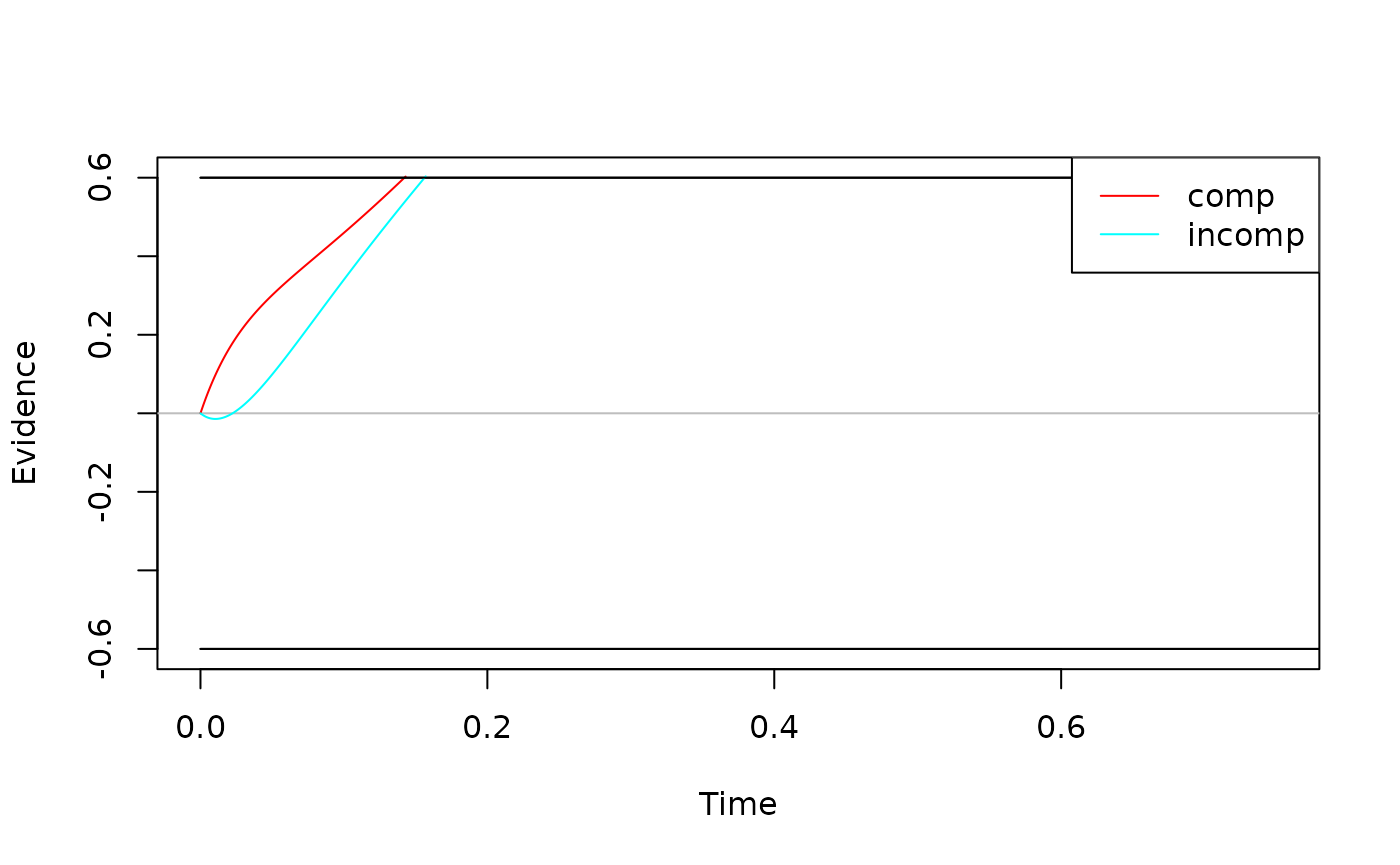
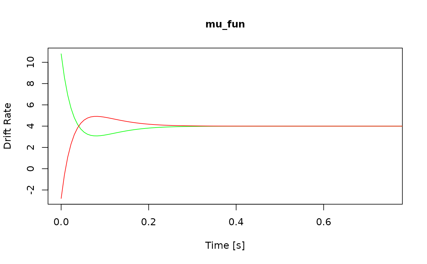
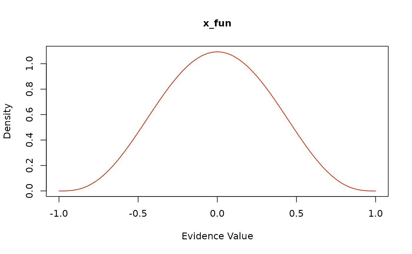
Alternatively, you can plot the returned values of each component
function by passing the model object to the generic plot()
method:

Finally, if you know what the model predictions should look like, you
can request these model predictions using the calc_stats()
function.
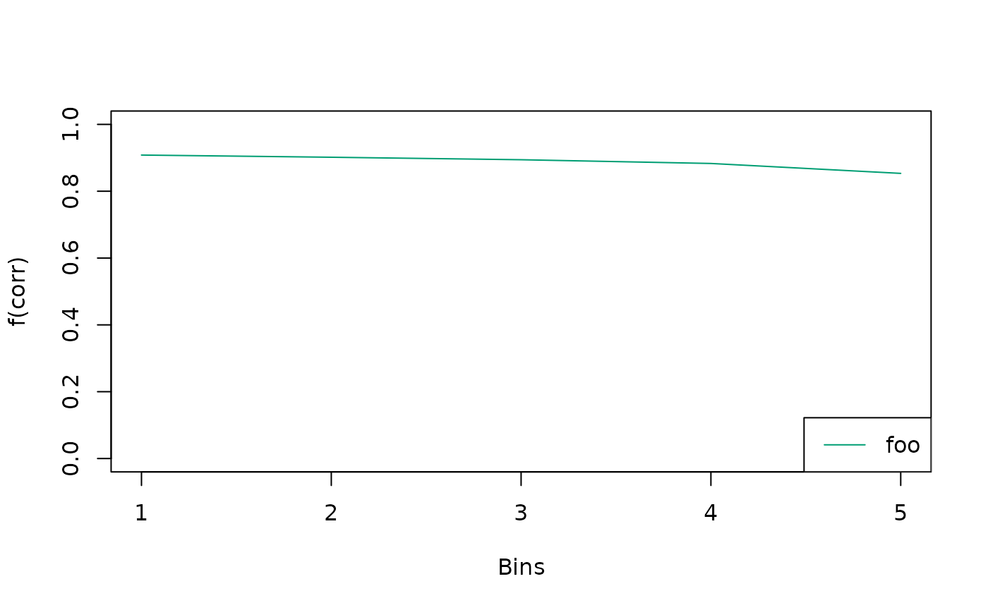
stats <- calc_stats(ddm, type = "quantiles")
plot(stats)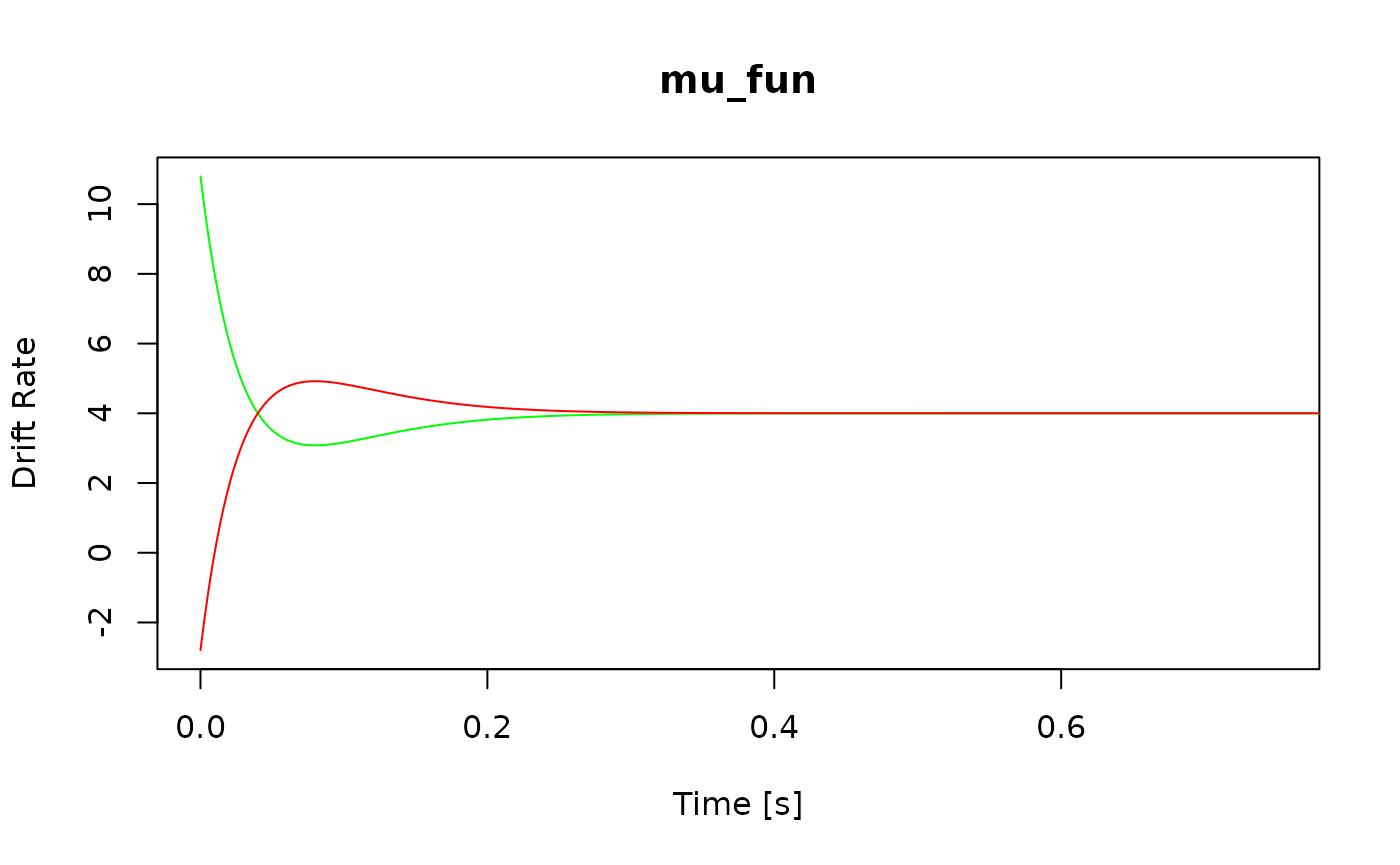
How do I choose values for dt and
dx?
By default, dRiftDM sets dt and
dx to 0.001, which is very conservative — we don’t know
which models you will create, so we’d rather be safe than sorry. In many
cases, though, these settings are unnecessarily small, leading to slow
evaluations and high computational burden. For the pre-built models, we
therefore use larger dt and dx values chosen
after extensive model simulations.
prms_solve(dmc_dm())
#>   sigma   t_max      dt      dx      nt      nx
#> 1.0e+00 3.0e+00 7.5e-03 2.0e-02 4.0e+02 1.0e+02
To help choose discretization settings, we provide
check_discretization(). It derives model predictions under
the current discretization and compares them to predictions obtained
under a fine discretization (with dx = dt =
0.001), separately for each condition, using the Hellinger distance.
cust_model <- cust_model() # some custom model
# set the intended discretization setting
prms_solve(cust_model)["dx"] <- .01
prms_solve(cust_model)["dt"] <- .005

# compare to a precise solution
check_discretization(cust_model)
#>     foo
#> 0.00859
The result is a per-condition deviance measure. If the predictions match exactly under both coarse and fine discretizations, the value is 0; if they are completely different, the value is 1. As a rule of thumb, we recommend keeping the deviance well below 5% for the parameter values that matter.
With check_discretization() in hand, it’s
straightforward to write small loops to explore parameter values and
discretization settings.
In addition, we can run small model-recovery studies to assess how discretization affects the reliability of parameter estimates.
What if I need to access an arbitrary R object within a
component function? Since each component function is called by
dRiftDM at runtime, users don’t have direct control over
the values passed as arguments. However, we have implemented a backdoor
via the ddm_opts argument of each component function. This
allows you to inject arbitrary R objects and evaluate them at runtime if
necessary. The following (not very creative) example shows how to do
this.
First, we write a custom component function that prints the
ddm_opts argument to the console. We then attach the string
“Hello World” to a model via the ddm_opts() method, set the
custom component function, and see the corresponding console output
after calling re_evaluate().
cust_mu <- function(prms_model, prms_solve, t_vec, one_cond, ddm_opts) {
  print(ddm_opts) # print out the values of ddm_opts
  muc <- rep(prms_model[["muc"]], length(t_vec))
  return(muc)
}

a_model <- ratcliff_dm() # a dummy model for demonstration purpose
ddm_opts(a_model) <- "Hello World" # attach "Hello World" to the model
comp_funs(a_model)[["mu_fun"]] <- cust_mu # swap in the custom component function

# evaluate the model (which will evaluate the custom drift rate function with the user-defined R
# object for ddm_opts)
a_model <- re_evaluate_model(a_model)
#> [1] "Hello World"
Because R is dynamic, we can attach arbitrary R objects and even
functions to the model via ddm_opts and thereby make them
available within our custom component functions.
Remark: Trial-by-Trial Variability in the Drift Rate
dRiftDM supports trial-by-trial variability in the drift rate for models with a time-independent (within-trial) drift rate. Its implementation is slightly different, however, as there is no dedicated model component for this feature. Instead, while solving the model, dRiftDM systematically increases and decreases the drift rate parameter to derive the first-passage-time distribution five times with different drift rates, and then averages across these distributions. As a consequence, we should expect computation time to increase by roughly a factor of five.
Two ingredients are required:
- we need a model with the
mu_constantcomponent function
- we need to add the parameter
sd_mucto the model. This internally triggers trial-by-trial variability in the drift rate
The following code shows how to create such a model. We can replace
any of the component functions or parameters, except those related to
mu_constant and mu_int_constant.
cust_model <- function() {
  # define all parameters and conditions
  prms_model <- c(
    non_dec = .2, # parameters for the non-decision time
    muc = 3, # parameter for a time-independent drift rate
    sd_muc = 1.2, # will trigger trial-by-trial variability in the drift rate!
    b = .4 # parameter for a time-independent boundary
  )

  # each model must have a condition
  # (in this example it is not relevant, so we just call it "foo")
  conds <- c("foo")

  # get access to pre-built component functions
  comps <- component_shelf()

  # call the drift_dm function which is the backbone of dRiftDM
  ddm <- drift_dm(
    prms_model = prms_model,
    conds = conds,
    subclass = "my_custom_model",
    mu_fun = comps$mu_constant, # time-independent drift rate with parameter muc
    mu_int_fun = comps$mu_int_constant, # respective integral of the drift rate
    x_fun = comps$x_dirac_0, # dirac delta on zero
    b_fun = comps$b_constant, # time-independent boundary b
    dt_b_fun = comps$dt_b_constant, # respective derivative of the boundary
    nt_fun = comps$nt_constant # time-independent non-decision time
  )
  return(ddm)
}

my_model <- cust_model()

# simulate some traces
set.seed(1)
plot(
  simulate_traces(my_model, k = 10, sigma = 0)
)
# visualize the effect of trial-by-trial variability: slow errors
plot(
  calc_stats(my_model, type = "cafs")
)