Introduction to dRiftDM

When working with drift-diffusion models (DDMs) you probably want to:

• Build a new model or select an existing model

• Explore the model behavior and validate that model parameters are estimated reliably

• Fit the model to data

• Explore the model fit

The dRiftDM package helps you to do this:

• With dedicated functions and workflows

• Options to customize models

• With efficient algorithms to derive the model predictions for time-dependent DDMs (see Richter, Ulrich, and Janczyk 2023)

Three pre-built models are currently available:

• The Ratcliff Diffusion Model (see ratcliff_dm(), Ratcliff 1978)

• The Diffusion Model for Conflict Tasks (see dmc_dm(), Ulrich et al. 2015; Janczyk, Mackenzie, and Koob 2024)

• The Shrinking Spotlight Model (see ssp_dm(), White, Ratcliff, and Starns 2011)

This document introduces you to dRiftDM, focusing on first steps in exploring and fitting a DDM.

An Examplary Model

To explore some of the basic functions of dRiftDM, we’ll use the Diffusion Model for Conflict Tasks (DMC). It is a diffusion model commonly employed in the context of cognitive psychology. To create the model, we call the pre-built function dmc_fun() and assign its output to a variable:

ddm <- dmc_dm()

Basic Properties of a Model

When printing a model to the console, we obtain detailed information about it:

print(ddm)
#> Class(es) dmc_dm, drift_dm
#> (model has not been estimated yet)
#> 
#> Parameter Values:
#>        muc   b non_dec sd_non_dec  tau a    A alpha
#> comp     4 0.6     0.3       0.02 0.04 2  0.1     4
#> incomp   4 0.6     0.3       0.02 0.04 2 -0.1     4
#> 
#> Parameter Settings:
#>        muc b non_dec sd_non_dec tau a A alpha
#> comp   1   2 3       4          5   0 6 7    
#> incomp 1   2 3       4          5   0 d 7    
#> 
#> Special Dependencies:
#> A ~ incomp == -(A ~ comp)
#> 
#> Custom Parameters:
#>        peak_l
#> comp     0.04
#> incomp   0.04
#> 
#> Deriving PDFS:
#>   solver: kfe
#>   values: sigma=1, t_max=3, dt=0.0075, dx=0.02, nt=400, nx=100
#> 
#> Cost Function: neg_log_like
#> 
#> Observed Data: NULL

Here we get a glimpse on the underlying structure of any model created with dRiftDM. For DMC this is:

• The model is of type dmc_dm

• The model has the parameters muc, b, …, alpha, and the current parameter values for each conditions are shown under Parameter Values. The conditions are comp and incomp in this case.

• Below this, under Parameter Settings, we obtain how each parameter behaves across conditions. If a number is the same for a parameter across conditions, this means that this parameter is equated across conditions. For example, the parameter muc is assumed to be identical for the conditions comp and incomp. If a number is zero, this means that this parameter is assumed to be “fixed” and thus is not a “free” parameter that can be estimated. If an entry shows a “d”, this means there is a special dependency, as listed under Special Dependencies (see vignette("customize_ddms", "dRiftDM") for more information).

• When fitting or exploring a model, we will have to derive the model predictions in terms of the first-passage-times (i.e., the duration of central response selection in the context of psychology). The settings for this are shown under Deriving PDFs. Currently, predictions are derived by a numerical discretization of the Kolmogorov-Forward-Equation (kfe). The diffusion constant sigma is 1, the maximum time space is 3 seconds, and the discretization in time and space is done in steps of .0075 and .02, respectively.

• Finally, under Cost Function, we can see the goal function that is used to compare observed data (not yet part of the model) and the model predictions. Per default, this cost function is the negative log-likelihood.

Exploring a Model

To explore a model, dRiftDM provides:

• simulate_traces() simulates realizations of the diffusion process

• calc_stats() calculates summary statistics of model predictions

simulate_traces()

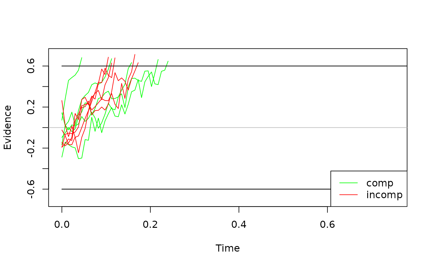
Realizations of a diffusion process, that is, single evidence accumulation traces for central response selection, are common ways to visualize a diffusion model. The first argument requires the model object. The second argument requires the number of realizations to simulate.

For example, we could simulate 5 traces for DMC per condition:

five_traces <- simulate_traces(object = ddm, k = 5)
five_traces
#> Class(es): traces_dm_list
#> 
#> Time space:
#> 0.000, 0.007, 0.015, 0.022 ... 3.000 
#> 
#> Condition: comp 
#> ~>  0.000, -0.040,  0.046, -0.113 ...  0.664 
#> ~>  0.000,  0.008, -0.011,  0.129 ...  0.660 
#> ~>  0.000,  0.036,  0.174,  0.255 ...  0.634 
#> ~>  0.000,  0.020,  0.067,  0.184 ...  0.773 
#> ...
#> 
#> Condition: incomp 
#> ~>  0.000, -0.073, -0.105, -0.070 ...  0.656 
#> ~>  0.000,  0.048,  0.106,  0.087 ...  0.665 
#> ~>  0.000, -0.013,  0.023, -0.046 ...  0.621 
#> ~>  0.000,  0.015, -0.091, -0.080 ...  0.610 
#> ...

Per default, traces are simulated by assuming a fixed starting value of zero. To simulate traces with a variable starting point (if provided by model), we can set the argument add_x = TRUE:

five_traces <- simulate_traces(object = ddm, k = 5, add_x = TRUE)
five_traces
#> Class(es): traces_dm_list
#> 
#> Time space:
#> 0.000, 0.007, 0.015, 0.022 ... 3.000 
#> 
#> Condition: comp 
#> ~> -0.288, -0.141, -0.166, -0.188 ...  0.647 
#> ~> -0.168,  0.024, -0.022,  0.026 ...  0.633 
#> ~>  0.144,  0.018,  0.060,  0.150 ...  0.672 
#> ~>  0.072,  0.279,  0.460,  0.487 ...  0.682 
#> ...
#> 
#> Condition: incomp 
#> ~> -0.144, -0.178, -0.149, -0.097 ...  0.686 
#> ~> -0.192, -0.067, -0.054, -0.059 ...  0.632 
#> ~>  0.264,  0.023, -0.088,  0.014 ...  0.630 
#> ~> -0.024, -0.078, -0.165, -0.167 ...  0.679 
#> ...

In the context of DMC, starting values of the traces are drawn from a symmetric beta distribution (see Ulrich et al. 2015).

We can easily visualize these traces by calling the generic plot() method:

plot(five_traces, col = c("green", "red"))

If you would like diffusion processes with a higher temporal resolution (e.g., for a nice publication-ready figure), simply increase dt (see the next chapter below) and run simulate_traces() once more.

When visualizing the basic model behavior, one sometimes wants to display the expected time-course of the diffusion process. We can do so by eliminating the stochastic noise with setting the argument sigma = 0.

exp_behavior <- simulate_traces(object = ddm, k = 1, sigma = 0)
plot(exp_behavior, col = c("green", "red"))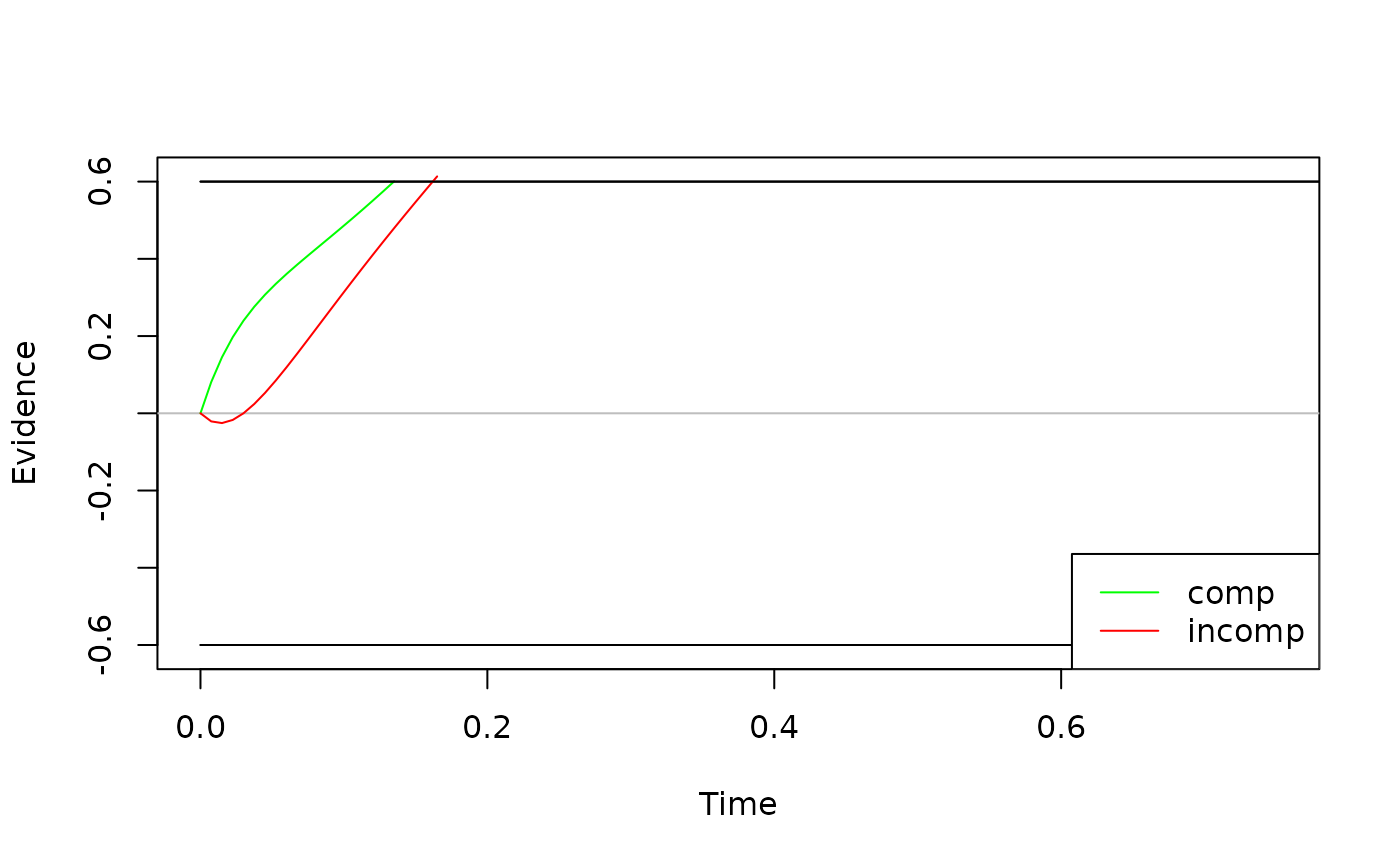

Note: When deriving the diffusion processes, dRiftDM simply uses the Euler-Maruyama method with a fixed time step size of dt. When actually deriving model predictions via the Kolmogorov-Forward-Equation, however, dRiftDM uses a dynamic time-stepping scheme to ensure high numerical accuracy even with relatively coarse settings for dt. Thus, if the model’s drift rate varies strongly and dt is large, the expected time course via simulate_traces() might not match the predicted model behavior.

calc_stats()

A DDM predicts response choices and response times, with the latter being the sum of the first-passage-time (i.e., the duration of central response selection) and the non-decision time. We can request summary statistics of this prediction with calc_stats(). The first argument requires the model object. The second argument a character vector, specifying the type of summary statistic.

In the context of cognitive psychology, quantiles and so-called Conditional Accuracy Functions (CAFs) are common ways to summarize the model predictions:

sum_stats <- calc_stats(object = ddm, type = c("cafs", "quantiles"))
sum_stats
#> Element 1, contains cafs
#> 
#>    Source   Cond Bin P_corr
#> 1    pred   comp   1  0.983
#> 2    pred   comp   2  0.983
#> 3    pred   comp   3  0.981
#> 4    pred   comp   4  0.984
#> 5    pred   comp   5  0.989
#> 6    pred incomp   1  0.835
#> 7    pred incomp   2  0.971
#> 8    pred incomp   3  0.986
#> 9    pred incomp   4  0.991
#> 10   pred incomp   5  0.992
#> 
#> 
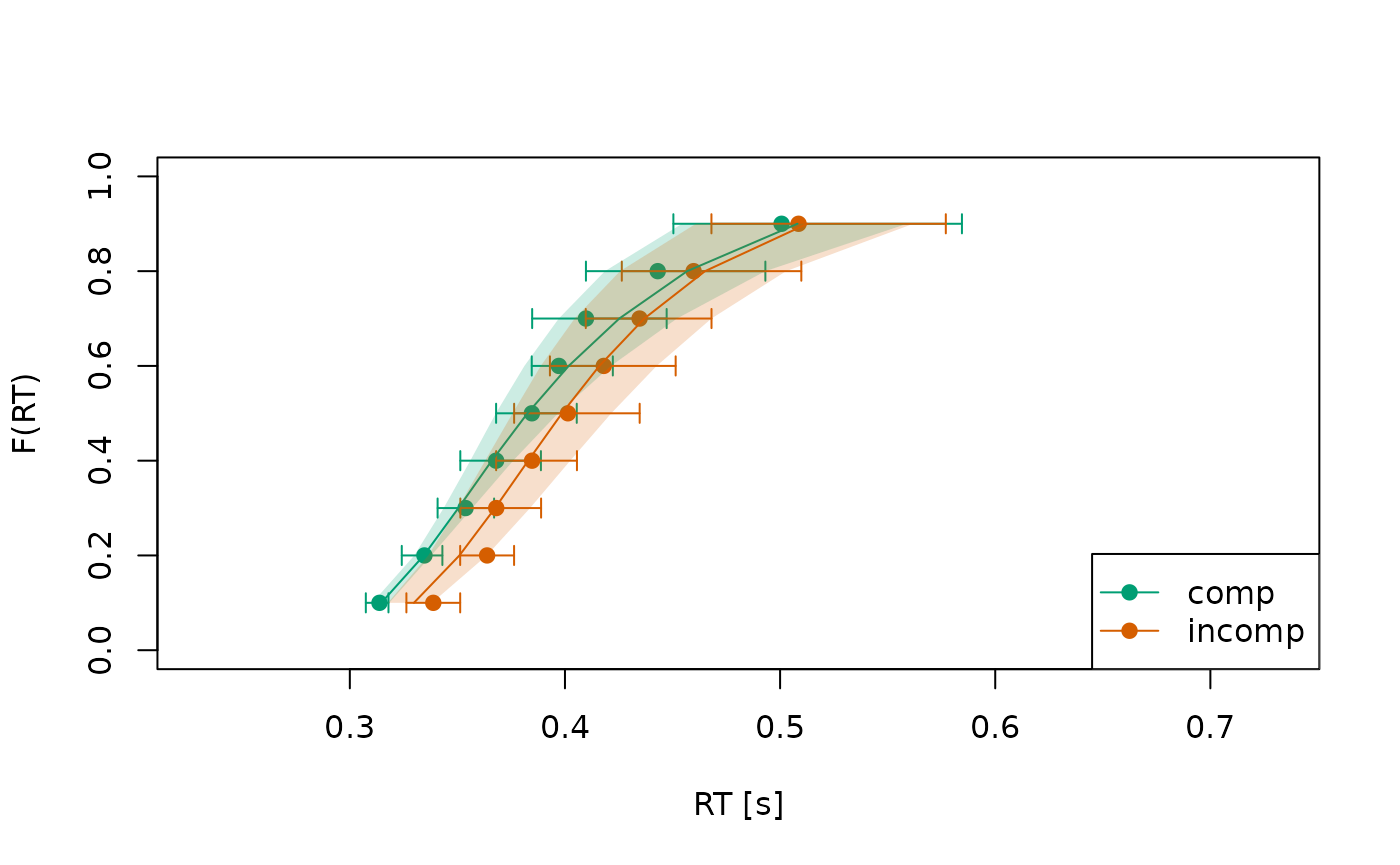
#> Element 2, contains quantiles
#> 
#>    Source   Cond Prob Quant_corr Quant_err
#> 1    pred   comp  0.1      0.325     0.321
#> 2    pred   comp  0.2      0.346     0.343
#> 3    pred   comp  0.3      0.364     0.362
#> 4    pred   comp  0.4      0.384     0.380
#> 5    pred   comp  0.5      0.406     0.398
#> 6    pred   comp  0.6      0.433     0.419
#> 7    pred   comp  0.7      0.465     0.443
#> 8    pred   comp  0.8      0.507     0.476
#> 9    pred   comp  0.9      0.574     0.531
#> 10   pred incomp  0.1      0.352     0.301
#> ...
#> 
#> (extract the list's elements as usual, e.g., with $cafs)

We can visualize summary statistics with the plot() method:

plot(sum_stats)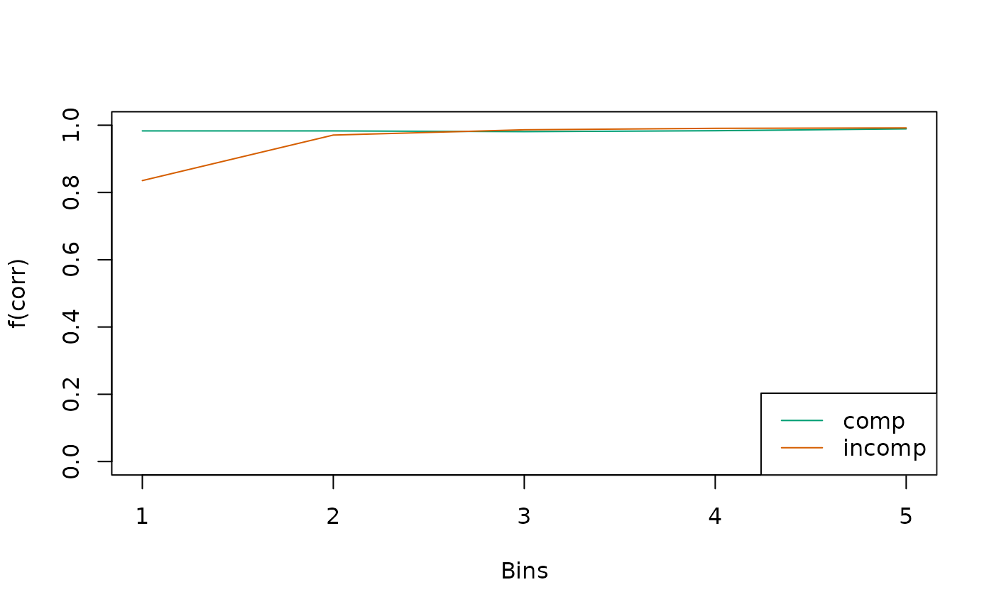

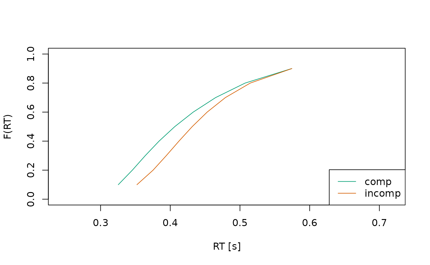
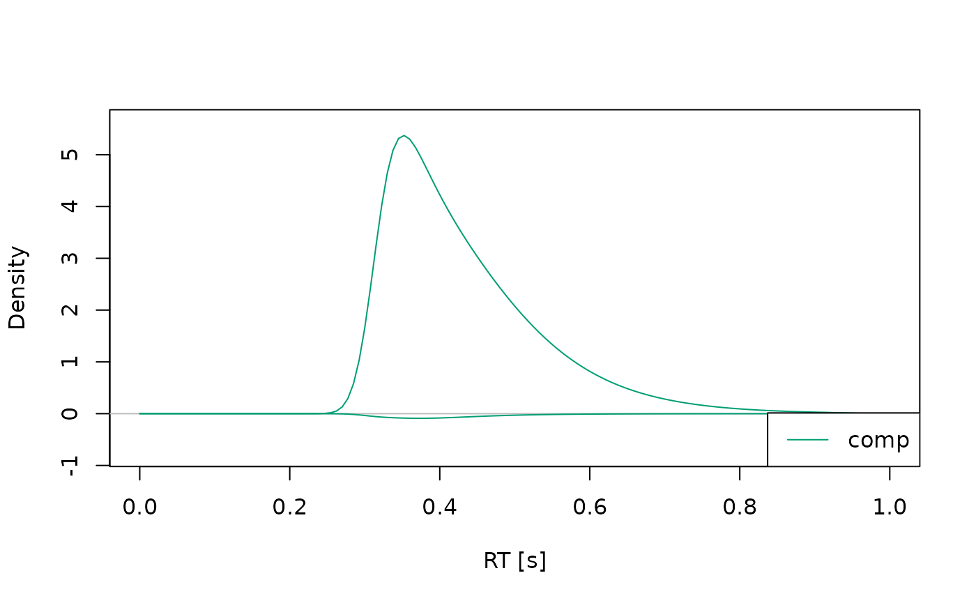
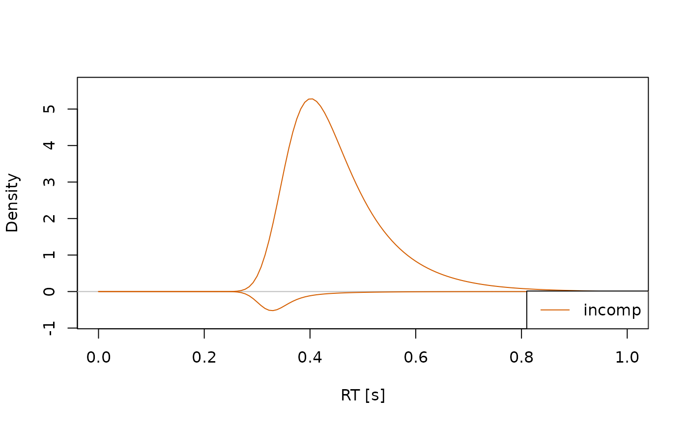
It is also possible to plot the predicted response time distributions using type = "densities".

sum_stats <- calc_stats(object = ddm, type = c("densities"))
sum_stats
#> Type of Statistic: densities
#> 
#>    Source Cond Stat  Time Dens_corr Dens_err
#> 1    pred comp  pdf 0.000         0        0
#> 2    pred comp  pdf 0.007         0        0
#> 3    pred comp  pdf 0.015         0        0
#> 4    pred comp  pdf 0.022         0        0
#> 5    pred comp  pdf 0.030         0        0
#> 6    pred comp  pdf 0.038         0        0
#> 7    pred comp  pdf 0.045         0        0
#> 8    pred comp  pdf 0.052         0        0
#> 9    pred comp  pdf 0.060         0        0
#> 10   pred comp  pdf 0.068         0        0
#> ...
#> 
#> (access the data.frame's columns/rows as usual)

In this case, it’s often helpful to plot the distributions separately for each condition, so they don’t overlap too much:

plot(sum_stats, conds = "comp", xlim = c(0, 1.0))

plot(sum_stats, conds = "incomp", xlim = c(0, 1.0))

Changing Model Properties

To get or set properties of the model, dRiftDM provides accessor/replacement methods for:

• coef() accesses/replaces parameter values

• prms_solve() accesses/replaces settings for deriving model predictions (this also includes changing the diffusion constant)

• solver() accesses/replaces the method for deriving model predictions (not really necessary anymore, the default kfe is well enough!)

• b_coding() accesses/replaces the coding of the upper and lower boundary

• obs_data() accesses/replaces the data set (of a single participant) attached to the model

• flex_prms() accesses/replaces the object that controls how each parameter relates across conditions

• conds() accesses/replaces the conditions of a model

• comp_funs() accesses/replaces the underlying component functions for the drift rate, boundary, etc.

• cost_function() accesses/replace the cost function used for parameter optimization.

Note: comp_funs(), flex_prms(), and conds() are covered in vignette("customize_ddms", "dRiftDM").

coef()

coef(ddm)
#>        muc          b    non_dec sd_non_dec        tau          A      alpha 
#>       4.00       0.60       0.30       0.02       0.04       0.10       4.00

This returns a unique representation of the parameters and their associated values. Note that this drops parameters that are not estimable.

We can combine coef() with the [] operator to change the values of the parameters:

coef(ddm)["muc"] <- 5
coef(ddm)
#>        muc          b    non_dec sd_non_dec        tau          A      alpha 
#>       5.00       0.60       0.30       0.02       0.04       0.10       4.00

To request the entire parameter matrix with all parameter values across conditions, we can set the argument select_unique = FALSE:

coef(ddm, select_unique = FALSE)
#>        muc   b non_dec sd_non_dec  tau a    A alpha peak_l
#> comp     5 0.6     0.3       0.02 0.04 2  0.1     4   0.04
#> incomp   5 0.6     0.3       0.02 0.04 2 -0.1     4   0.04

In this case, we can not combine coef() with the [] operator. To change a parameter value for a specific condition, we can use the function modify_flex_prms().

prms_solve()

prms_solve(ddm)
#>   sigma   t_max      dt      dx      nt      nx 
#> 1.0e+00 3.0e+00 7.5e-03 2.0e-02 4.0e+02 1.0e+02

This shows the diffusion constant and the discretization settings. We can again use a combination with [] to modify these values.

prms_solve(ddm)["dt"] <- .005
prms_solve(ddm)
#> sigma t_max    dt    dx    nt    nx 
#> 1e+00 3e+00 5e-03 2e-02 6e+02 1e+02

Remark: Discretization Settings

Setting the discretization, in particluar for dt and dx, is a tricky choice. If you create a new model (see the vignette("customize_ddms", "dRiftDM")), dRiftDM discretizes the time and evidence space in steps of dx = dt = 0.001. This is a very conservative setting, ensuring high numerical accuracy for many DDMs. Yet, this high numerical accuracy comes at the expense of a high computational burden that increases non-linearly.

For the models that are pre-built (i.e., for dmc_dm(), ssp_dm(), and ratcliff_dm()), we have conducted extensive simulations to find a discretization that provides a good balance between speed and accuracy. However, these settings will not hold for all models that you might create with dRiftDM. It is thus highly recommended for custom models to perform some exploratory model simulations under different discretization and parameter setttings. As a rule of thumb, we currently recommend exploring dt values between 0.001 and 0.01, and dx values between 0.001 and 0.02.

Another choice is the maximum time space. It should be large enough to easily cover the longest response time in the observed data set.

A helpful function to check the impact of the discretization setting, in particular for dt and dx is the check_discretization() function. This function takes a model (with some values for dt and dx) and compares the model predictions with these settings against model predictions obtained under very fine discretization settings using the Hellinger-Distance.

check_discretization(ddm)
#>    comp  incomp 
#> 0.01027 0.01431

we can interpret the result as a percentage of deviance. If the model predictions under fine and a more coarse settings are exactly the same, the returned values will be zero. If they are completely different, they will be one. From our own (yet preliminary) experience, we would recommend keeping the Hellinger Distance clearly below 5 percent for most of the relevant parameter settings.

solver()

solver(ddm)
#> [1] "kfe"

This shows the currently set method for deriving the model’s predicted probability density functions of response time and choice. Currently supported options are "kfe" and "im_zero". While the "kfe" method can be applied to all models in dRiftDM, "im_zero" can only be used when the starting point is fixed to zero. Also, "im_zero" currently doesn’t support adaptive time stepping, and requires finer discretization. Thus, for now, "im_zero" is only present for backward compatibility, and we recommend using the "kfe" solver.

b_coding()

b_coding(ddm)
#> $column
#> [1] "Error"
#> 
#> $u_name_value
#> corr 
#>    0 
#> 
#> $l_name_value
#> err 
#>   1

This returns a list that specifies how the boundaries of a DDM are coded. We can change the boundary coding by modifying the returned list:

copy <- ddm # to not change the original model object
b_coding(copy)$column <- "Response"
b_coding(copy)$u_name_value <- c("left" = -1)
b_coding(copy)$l_name_value <- c("right" = 1)

b_coding(copy)
#> $column
#> [1] "Response"
#> 
#> $u_name_value
#> left 
#>   -1 
#> 
#> $l_name_value
#> right 
#>     1

Changing the boundary coding makes sense if the response choices of your observed data is not accuracy coded.

Note that this will also alter the column names of the summary statistics:

calc_stats(copy, "quantiles")
#> Type of Statistic: quantiles
#> 
#>    Source   Cond Prob Quant_left Quant_right
#> 1    pred   comp  0.1      0.321       0.310
#> 2    pred   comp  0.2      0.339       0.327
#> 3    pred   comp  0.3      0.355       0.342
#> 4    pred   comp  0.4      0.371       0.357
#> 5    pred   comp  0.5      0.388       0.373
#> 6    pred   comp  0.6      0.408       0.390
#> 7    pred   comp  0.7      0.433       0.409
#> 8    pred   comp  0.8      0.466       0.435
#> 9    pred   comp  0.9      0.517       0.476
#> 10   pred incomp  0.1      0.345       0.297
#> ...
#> 
#> (access the data.frame's columns/rows as usual)

obs_data()

We can set observed data of a single individual to a model (or access it) with obs_data(). When setting observed data, we have to make sure that the supplied data.frame provides columns matching with the boundary coding and the conditions of the model.

data <- dRiftDM::dmc_synth_data # some synthetic data suitable for DMC that ships with dRiftDM
# the Cond column matches with conds(ddm).
# The Error column matches b_coding(ddm)
# the RT column is in seconds ;)
head(data)
#>      RT Error Cond
#> 1 0.349     0 comp
#> 2 0.444     0 comp
#> 3 0.441     0 comp
#> 4 0.572     0 comp
#> 5 0.438     0 comp
#> 6 0.535     0 comp

obs_data(ddm) <- data

Note that the supplied data set is not stored “as is” within the model object. Thus, when accessing a data set of a model, the data is re-assembled, and this might change the order of rows or column with respect to the original data set. To remind you of that, a message is thrown.

extr_data <- obs_data(ddm)
#> Extracting observed data from a model object. Remember that the result may be sorted differently than expect!
head(extr_data)
#>      RT Error Cond
#> 1 0.349     0 comp
#> 2 0.444     0 comp
#> 3 0.441     0 comp
#> 4 0.572     0 comp
#> 5 0.438     0 comp
#> 6 0.535     0 comp

The summary() Function

We can request a detailed summary of the model, providing information about it’s core properties with the generic summary() function:

summary(ddm)
#> Class(es) dmc_dm, drift_dm
#> 
#> Parameter Values:
#>        muc   b non_dec sd_non_dec  tau a    A alpha
#> comp     5 0.6     0.3       0.02 0.04 2  0.1     4
#> incomp   5 0.6     0.3       0.02 0.04 2 -0.1     4
#> 
#> Parameter Settings:
#>        muc b non_dec sd_non_dec tau a A alpha
#> comp   1   2 3       4          5   0 6 7    
#> incomp 1   2 3       4          5   0 d 7    
#> 
#> Special Dependencies:
#> A ~ incomp == -(A ~ comp)
#> 
#> Custom Parameters:
#>        peak_l
#> comp     0.04
#> incomp   0.04
#> 
#> Observed Data:
#>              min. 1st qu. median  mean 3rd qu.  max.   n
#> corr comp   0.331   0.436  0.479 0.507   0.549 1.075 292
#> corr incomp 0.313   0.474  0.528 0.543   0.592 0.879 268
#> err comp    0.428   0.458  0.526 0.564   0.621 0.871   8
#> err incomp  0.302   0.398  0.452 0.458   0.498 0.771  32
#> 
#> Fit Indices:
#>     Log_Like Neg_Log_Like          AIC          BIC       RMSE_s      RMSE_ms 
#>     -180.145      180.145      374.290      405.069        0.107      106.502 
#> 
#> -------
#> Deriving PDFS:
#>   solver: kfe
#>   values: sigma=1, t_max=3, dt=0.005, dx=0.02, nt=600, nx=100
#> 
#> Boundary Coding:
#>   upper: corr 
#>   lower: err 
#>   expected data column: Error (corr = 0; err = 1)

Fitting a Model

To fit a model to observed data we can use estimate_dm(). We can choose between:

• Fitting a model separately to multiple participants using classical optimization (i.e., minimizing a cost function)

• Fitting a model to aggregated data (i.e., first aggregate data across individuals and then fit the model once by minimizing a cost function based on summary statistics)

• Fitting a model separately to multiple participants using Bayesian estimation (i.e., explore the posterior distribution using Markov-Chain Monte-Carlo; experimental)

• Fitting a model hierarchically using Bayesian estimation (experimental)

Fitting a Model Separately to Individual Data Using Classical Optimization Techniques

Given a data set, the parameters of a model in dRiftDM are estimated via Differential Evolution, (bounded) Nelder-Mead, or (bounded) Broyden-Fletcher-Goldfarb-Shanno. The cost function is based either on the log-likelihood or the Root-Mean-Squared-Error (RMSE) statistic.

The first argument drift_dm_obj requires the model. The second argument obs_data requires some observed data with 4 columns:

• ID: an identifier, coding the different individuals
• RT: observed response times in seconds
• Error: observed errors/choices per trial (remember that this column and its values must match with the boundary coding of your model!)
• Cond: the conditions of each trial (within-participants only; must match with the conditions of your model)

drift_dm_obj and obs_data are the only mandatory arguments! However, as we will see in a second, specifying some of the remaining arguments is often highly recommended. For demonstration purpose, we will fit the first four individuals of the Simon data set provided by Ulrich et al. (2015).

# get some data (here we use a Simon data set provided by Ulrich et al.)
data <- dRiftDM::ulrich_simon_data
data <- data[data$ID %in% 1:4, ] # just the first four individuals

# get a model (here we again use the pre-built DMC model)
ddm <- dmc_dm()

# the provided data is ready-to-use with DMC
head(data)
#>   ID        RT Error   Cond
#> 1  1 0.4514001     0 incomp
#> 2  1 0.5348854     0 incomp
#> 3  1 0.4680900     0 incomp
#> 4  1 0.4346847     0   comp
#> 5  1 0.3847005     0   comp
#> 6  1 0.4347649     0 incomp

# now call the estimation routine
all_fits <- estimate_dm(
  drift_dm_obj = ddm,
  obs_data = data,
  verbose = 1 # prints more information about the underlying optimization run
)
#> Using the data supplied via the 'obs_data' argument.
#> Using optimizer 'Nelder-Mead'.
#> Fitting the model separately to multiple participants (cost function:'neg_log_like'). The result will be a fit object of type 'fits_ids_dm'.
#> Using EZ-Diffusion estimates for: muc, b, non_dec
#> Performing latin hypercube sampling (n_lhs = 10) on: sd_non_dec, tau, A, alpha
#> Starting optimizer 'Nelder-Mead' with the following starting values:
#> muc=3.936, b=0.39, non_dec=0.306, sd_non_dec=0.027, tau=0.059, A=0.074, alpha=7.498
#> Warning in estimate_classical(drift_dm_obj = one_model_start$drift_dm_obj, :
#> The optimization routine did not converge successfully (convergence message:
#> maxit reached). Treat the estimated parameters with some caution.
#> Optimization routine exited after 502 function evaluations
#> Final Parameters:
#> muc = 4.263
#> b = 0.438
#> non_dec = 0.307
#> sd_non_dec = 0.029
#> tau = 0.025
#> A = 0.088
#> alpha = 8.185
#> ==> gave a neg_log_like of -419.191
#> Using EZ-Diffusion estimates for: muc, b, non_dec
#> Performing latin hypercube sampling (n_lhs = 10) on: sd_non_dec, tau, A, alpha
#> Starting optimizer 'Nelder-Mead' with the following starting values:
#> muc=3.512, b=0.379, non_dec=0.287, sd_non_dec=0.041, tau=0.069, A=0.036, alpha=6.628
#> Warning in estimate_classical(drift_dm_obj = one_model_start$drift_dm_obj, :
#> The optimization routine did not converge successfully (convergence message:
#> maxit reached). Treat the estimated parameters with some caution.
#> Optimization routine exited after 502 function evaluations
#> Final Parameters:
#> muc = 4.147
#> b = 0.383
#> non_dec = 0.302
#> sd_non_dec = 0.032
#> tau = 0.064
#> A = 0.049
#> alpha = 5.273
#> ==> gave a neg_log_like of -383.355
#> Using EZ-Diffusion estimates for: muc, b, non_dec
#> Performing latin hypercube sampling (n_lhs = 10) on: sd_non_dec, tau, A, alpha
#> Starting optimizer 'Nelder-Mead' with the following starting values:
#> muc=4.759, b=0.443, non_dec=0.292, sd_non_dec=0.022, tau=0.16, A=0.033, alpha=5.641
#> Warning in estimate_classical(drift_dm_obj = one_model_start$drift_dm_obj, :
#> The optimization routine did not converge successfully (convergence message:
#> maxit reached). Treat the estimated parameters with some caution.
#> Optimization routine exited after 502 function evaluations
#> Final Parameters:
#> muc = 5.617
#> b = 0.467
#> non_dec = 0.302
#> sd_non_dec = 0.021
#> tau = 0.011
#> A = 0.052
#> alpha = 6.718
#> ==> gave a neg_log_like of -510.38
#> Using EZ-Diffusion estimates for: muc, b, non_dec
#> Performing latin hypercube sampling (n_lhs = 10) on: sd_non_dec, tau, A, alpha
#> Starting optimizer 'Nelder-Mead' with the following starting values:
#> muc=2.187, b=0.497, non_dec=0.27, sd_non_dec=0.029, tau=0.218, A=0.03, alpha=6.945
#> Warning in estimate_classical(drift_dm_obj = one_model_start$drift_dm_obj, :
#> The optimization routine did not converge successfully (convergence message:
#> maxit reached). Treat the estimated parameters with some caution.
#> Optimization routine exited after 502 function evaluations
#> Final Parameters:
#> muc = 2.651
#> b = 0.501
#> non_dec = 0.292
#> sd_non_dec = 0.038
#> tau = 0.055
#> A = 0.049
#> alpha = 5.745
#> ==> gave a neg_log_like of -165.915
#> Warning in estimate_classical_wrapper(drift_dm_obj = drift_dm_obj, obs_data_ids = obs_data, : The optimization routine did not converge successfully for the following IDs: 1, 2, 3, 4
#> Summary of messages:
#> - maxit reached

From the messages, it becomes clear that dRiftDM used the “Nelder-Mead” optimization algorithm to minimize the negative log-likelihood. The starting values were taken from the model:

coef(ddm)
#>        muc          b    non_dec sd_non_dec        tau          A      alpha 
#>       4.00       0.60       0.30       0.02       0.04       0.10       4.00

However, while the code runs, it threw convergence warnings for each individual. Thus, while searching for the “optimal” parameters, the optimization algorithm could not find a clear minimum after 502 function evaluations. To get rid of the convergence warning, we could:

1. Switch the optimization algorithm
2. Let the optimization algorithm search for a longer period.

Let’s try the second option first. To configure the settings of an optimization algorithm, we can use the control argument (which is ultimately passed forward to stats::optim() in this case; see the documentation of estimate_dm() for more info).

all_fits <- estimate_dm(
  drift_dm_obj = ddm,
  obs_data = data,
  control = list(maxit = 2000), # 2000 iterations; see stats::optim
  verbose = 1 # more information about the underlying optimization run
)
#> Using the data supplied via the 'obs_data' argument.
#> Using optimizer 'Nelder-Mead'.
#> Fitting the model separately to multiple participants (cost function:'neg_log_like'). The result will be a fit object of type 'fits_ids_dm'.
#> Using EZ-Diffusion estimates for: muc, b, non_dec
#> Performing latin hypercube sampling (n_lhs = 10) on: sd_non_dec, tau, A, alpha
#> Starting optimizer 'Nelder-Mead' with the following starting values:
#> muc=3.936, b=0.39, non_dec=0.306, sd_non_dec=0.025, tau=0.238, A=0.074, alpha=7.407
#> Optimization routine exited after 1104 function evaluations
#> Final Parameters:
#> muc = 4.288
#> b = 0.409
#> non_dec = 0.315
#> sd_non_dec = 0.035
#> tau = 0.023
#> A = 0.09
#> alpha = 9.046
#> ==> gave a neg_log_like of -417.937
#> Using EZ-Diffusion estimates for: muc, b, non_dec
#> Performing latin hypercube sampling (n_lhs = 10) on: sd_non_dec, tau, A, alpha
#> Starting optimizer 'Nelder-Mead' with the following starting values:
#> muc=3.512, b=0.379, non_dec=0.287, sd_non_dec=0.027, tau=0.075, A=0.017, alpha=5.836
#> Optimization routine exited after 1041 function evaluations
#> Final Parameters:
#> muc = 4.26
#> b = 0.378
#> non_dec = 0.305
#> sd_non_dec = 0.032
#> tau = 0.061
#> A = 0.018
#> alpha = 4.321
#> ==> gave a neg_log_like of -382.68
#> Using EZ-Diffusion estimates for: muc, b, non_dec
#> Performing latin hypercube sampling (n_lhs = 10) on: sd_non_dec, tau, A, alpha
#> Starting optimizer 'Nelder-Mead' with the following starting values:
#> muc=4.759, b=0.443, non_dec=0.292, sd_non_dec=0.019, tau=0.218, A=0.094, alpha=6.858
#> Optimization routine exited after 1286 function evaluations
#> Final Parameters:
#> muc = 5.177
#> b = 0.404
#> non_dec = 0.307
#> sd_non_dec = 0.018
#> tau = 0.012
#> A = 0.067
#> alpha = 15.44
#> ==> gave a neg_log_like of -512.195
#> Using EZ-Diffusion estimates for: muc, b, non_dec
#> Performing latin hypercube sampling (n_lhs = 10) on: sd_non_dec, tau, A, alpha
#> Starting optimizer 'Nelder-Mead' with the following starting values:
#> muc=2.187, b=0.497, non_dec=0.27, sd_non_dec=0.026, tau=0.055, A=0.08, alpha=6.095
#> Warning in estimate_classical(drift_dm_obj = one_model_start$drift_dm_obj, :
#> The optimization routine did not converge successfully (convergence message:
#> degeneracy of Nelder-Mead simplex). Treat the estimated parameters with some
#> caution.
#> Optimization routine exited after 316 function evaluations
#> Final Parameters:
#> muc = 2.878
#> b = 0.534
#> non_dec = 0.304
#> sd_non_dec = 0.035
#> tau = 0.043
#> A = 0.096
#> alpha = 2.832
#> ==> gave a neg_log_like of -172.065
#> Warning in estimate_classical_wrapper(drift_dm_obj = drift_dm_obj, obs_data_ids = obs_data, : The optimization routine did not converge successfully for the following IDs: 4
#> Summary of messages:
#> - degeneracy of Nelder-Mead simplex

Now the algorithm converges after about 600 to 1000 function evaluations.

What about the other option of switching the algorithm? Instead of using “Nelder-Mead”, we could use “nmkb”. The “nmkb” optimization algorithm is essentially “Nelder-Mead”, but it uses constraints on the parameters to search a more clearly defined space (which sometimes helps, but not always). We can request “nmkb” by using the arguments optimizer and lower/upper.

For lower/upper, we have to define ranges for each parameter that is considered free in at least one condition; essentially, this means we have to define a range for each of the following parameters:

coef(ddm)
#>        muc          b    non_dec sd_non_dec        tau          A      alpha 
#>       4.00       0.60       0.30       0.02       0.04       0.10       4.00

Fortunately, since dRiftDM v0.3.0 the function get_lower_upper() makes it easier to select these ranges—at least for the pre-built models and model components:

l_u <- get_lower_upper(ddm)
print(l_u)
#> $lower
#>        muc          b    non_dec sd_non_dec        tau          A      alpha 
#>     0.5000     0.1500     0.1500     0.0075     0.0150     0.0050     2.0000 
#> 
#> $upper
#>        muc          b    non_dec sd_non_dec        tau          A      alpha 
#>       9.00       1.20       0.60       0.10       0.25       0.30       8.00

all_fits_nmkb <- estimate_dm(
  drift_dm_obj = ddm,
  obs_data = data,
  optimizer = "nmkb",
  lower = l_u$lower,
  upper = l_u$upper,
  verbose = 1 # more information about the underlying optimization run
)
#> Using the data supplied via the 'obs_data' argument.
#> Using optimizer 'nmkb'.
#> Fitting the model separately to multiple participants (cost function:'neg_log_like'). The result will be a fit object of type 'fits_ids_dm'.
#> Using EZ-Diffusion estimates for: muc, b, non_dec
#> Performing latin hypercube sampling (n_lhs = 10) on: sd_non_dec, tau, A, alpha
#> Starting optimizer 'nmkb' with the following starting values:
#> muc=3.936, b=0.39, non_dec=0.306, sd_non_dec=0.025, tau=0.132, A=0.06, alpha=7.677
#> Optimization routine exited after 1315 function evaluations
#> Final Parameters:
#> muc = 4.21
#> b = 0.395
#> non_dec = 0.315
#> sd_non_dec = 0.029
#> tau = 0.08
#> A = 0.032
#> alpha = 7.415
#> ==> gave a neg_log_like of -414.813
#> Using EZ-Diffusion estimates for: muc, b, non_dec
#> Performing latin hypercube sampling (n_lhs = 10) on: sd_non_dec, tau, A, alpha
#> Starting optimizer 'nmkb' with the following starting values:
#> muc=3.512, b=0.379, non_dec=0.287, sd_non_dec=0.032, tau=0.015, A=0.037, alpha=7.887
#> Optimization routine exited after 732 function evaluations
#> Final Parameters:
#> muc = 4.046
#> b = 0.366
#> non_dec = 0.304
#> sd_non_dec = 0.033
#> tau = 0.015
#> A = 0.064
#> alpha = 7.951
#> ==> gave a neg_log_like of -384.096
#> Using EZ-Diffusion estimates for: muc, b, non_dec
#> Performing latin hypercube sampling (n_lhs = 10) on: sd_non_dec, tau, A, alpha
#> Starting optimizer 'nmkb' with the following starting values:
#> muc=4.759, b=0.443, non_dec=0.292, sd_non_dec=0.021, tau=0.209, A=0.122, alpha=5.36
#> Optimization routine exited after 1100 function evaluations
#> Final Parameters:
#> muc = 5.347
#> b = 0.439
#> non_dec = 0.304
#> sd_non_dec = 0.019
#> tau = 0.015
#> A = 0.066
#> alpha = 7.97
#> ==> gave a neg_log_like of -512.114
#> Using EZ-Diffusion estimates for: muc, b, non_dec
#> Performing latin hypercube sampling (n_lhs = 10) on: sd_non_dec, tau, A, alpha
#> Starting optimizer 'nmkb' with the following starting values:
#> muc=2.187, b=0.497, non_dec=0.27, sd_non_dec=0.013, tau=0.068, A=0.055, alpha=7.786
#> Optimization routine exited after 1082 function evaluations
#> Final Parameters:
#> muc = 2.871
#> b = 0.527
#> non_dec = 0.302
#> sd_non_dec = 0.036
#> tau = 0.057
#> A = 0.104
#> alpha = 2.839
#> ==> gave a neg_log_like of -172.3

In this case, we only saw a convergence warning for one participant. By increasing the number of iterations, this warning again disappears:

all_fits_nmkb <- estimate_dm(
  drift_dm_obj = ddm,
  obs_data = data,
  optimizer = "nmkb",
  lower = l_u$lower,
  upper = l_u$upper,
  control = list(maxfeval = 2000), # see dfoptim::nmkb
  verbose = 1 # more information about the underlying optimization run
)
#> Using the data supplied via the 'obs_data' argument.
#> Using optimizer 'nmkb'.
#> Fitting the model separately to multiple participants (cost function:'neg_log_like'). The result will be a fit object of type 'fits_ids_dm'.
#> Using EZ-Diffusion estimates for: muc, b, non_dec
#> Performing latin hypercube sampling (n_lhs = 10) on: sd_non_dec, tau, A, alpha
#> Starting optimizer 'nmkb' with the following starting values:
#> muc=3.936, b=0.39, non_dec=0.306, sd_non_dec=0.023, tau=0.104, A=0.066, alpha=7.879
#> Optimization routine exited after 1504 function evaluations
#> Final Parameters:
#> muc = 4.23
#> b = 0.411
#> non_dec = 0.314
#> sd_non_dec = 0.028
#> tau = 0.02
#> A = 0.093
#> alpha = 7.946
#> ==> gave a neg_log_like of -420.397
#> Using EZ-Diffusion estimates for: muc, b, non_dec
#> Performing latin hypercube sampling (n_lhs = 10) on: sd_non_dec, tau, A, alpha
#> Starting optimizer 'nmkb' with the following starting values:
#> muc=3.512, b=0.379, non_dec=0.287, sd_non_dec=0.033, tau=0.084, A=0.061, alpha=7.114
#> Optimization routine exited after 530 function evaluations
#> Final Parameters:
#> muc = 4.229
#> b = 0.381
#> non_dec = 0.305
#> sd_non_dec = 0.032
#> tau = 0.023
#> A = 0.053
#> alpha = 4.625
#> ==> gave a neg_log_like of -384.316
#> Using EZ-Diffusion estimates for: muc, b, non_dec
#> Performing latin hypercube sampling (n_lhs = 10) on: sd_non_dec, tau, A, alpha
#> Starting optimizer 'nmkb' with the following starting values:
#> muc=4.759, b=0.443, non_dec=0.292, sd_non_dec=0.015, tau=0.131, A=0.051, alpha=5.635
#> Optimization routine exited after 1160 function evaluations
#> Final Parameters:
#> muc = 5.27
#> b = 0.438
#> non_dec = 0.303
#> sd_non_dec = 0.018
#> tau = 0.054
#> A = 0.021
#> alpha = 7.557
#> ==> gave a neg_log_like of -510.464
#> Using EZ-Diffusion estimates for: muc, b, non_dec
#> Performing latin hypercube sampling (n_lhs = 10) on: sd_non_dec, tau, A, alpha
#> Starting optimizer 'nmkb' with the following starting values:
#> muc=2.187, b=0.497, non_dec=0.27, sd_non_dec=0.027, tau=0.213, A=0.039, alpha=7.117
#> Optimization routine exited after 805 function evaluations
#> Final Parameters:
#> muc = 2.901
#> b = 0.533
#> non_dec = 0.303
#> sd_non_dec = 0.037
#> tau = 0.053
#> A = 0.1
#> alpha = 2.862
#> ==> gave a neg_log_like of -172.311

When you provide lower/upper, the default is actually not “nmkb”, but “DEoptim”. The ‘DE’ stands for Differential Evolution—a slower but very robust optimization algorithm. If runtime is not critical, we recommend using “DEoptim”, since it performs reliably even when the cost function is complex (which is almost always the case with DDMs).

all_fits_deoptim <- estimate_dm(
  drift_dm_obj = ddm,
  obs_data = data,
  lower = l_u$lower,
  upper = l_u$upper,
  n_cores = 1 # you might want to increase this
)

Because DEoptim is time-consuming, it is recommended to use multiple cores. You can set the desired number of cores using the n_cores argument.¹ To get the number of available cores, use parallel::detectCores().

A common question concerns the number of cores to use. By default, dRiftDM (>v.0.3.0) parallelizes across individuals—that is, one individual is fitted per core. Therefore, you should not specify more cores than there are individuals. In the present toy example, this limits the number of cores to four.

Additionally, the fitting process runs in batches. For instance, if there are two cores and four individuals, dRiftDM first fits the first two individuals and then the remaining two. In practice, it is thus often convenient to choose a number of cores that divides the number of individuals evenly (e.g., six cores for 18 individuals, 50 cores for 200 individuals).

It is also possible to parallelize within individuals when using DEoptim (this is not the default). In this case, fitting a single individual uses multiple cores. This option can be useful when fitting only a few participants or when model evaluation is relatively slow (i.e., when dt and dx are small). Otherwise, the overhead of managing multiple cores outweighs the computational burden per core. We can choose among parallelization within and across individuals using the argument parallelization_strategy.

Remark: Fitting Just One Individual

In all previous examples, the function estimate_dm() returned an object of class fits_ids_dm, which contains all the individual fits.

# Example
class(all_fits_deoptim)
#> [1] "fits_ids_dm"
print(all_fits_deoptim)
#> Fit approach: separately - classical
#> Fitted model type: dmc_dm, drift_dm
#> Optimizer: DEoptim 
#> Convergence: NA 
#> N Individuals: 4 
#> Average Trial Numbers:
#>  167 trials comp; 168 trials incomp
#> Cost Function: neg_log_like

A special case occurs when fitting only a single individual. In this case, dRiftDM returns the model object itself, including the data and the updated parameters for that individual. This behavior is maintained for backward compatibility. Nothing special to worry about—just be aware of it.

ddm_est <- estimate_dm(
  drift_dm_obj = ddm,
  obs_data = data[data$ID == 1, ],
  optimizer = "Nelder-Mead",
  control = list(maxit = 2000),
  messaging = FALSE, verbose = 0 # just to reduce the amount of information shown
)
class(ddm_est)
#> [1] "dmc_dm"   "drift_dm"
print(ddm_est)
#> Class(es) dmc_dm, drift_dm
#> Optimizer: Nelder-Mead
#> Convergence: TRUE
#> 
#> Parameter Values:
#>         muc     b non_dec sd_non_dec   tau a      A alpha
#> comp   4.27 0.422   0.312      0.028 0.078 2  0.013 4.759
#> incomp 4.27 0.422   0.312      0.028 0.078 2 -0.013 4.759
#> 
#> Parameter Settings:
#>        muc b non_dec sd_non_dec tau a A alpha
#> comp   1   2 3       4          5   0 6 7    
#> incomp 1   2 3       4          5   0 d 7    
#> 
#> Special Dependencies:
#> A ~ incomp == -(A ~ comp)
#> 
#> Custom Parameters:
#>        peak_l
#> comp    0.078
#> incomp  0.078
#> 
#> Deriving PDFS:
#>   solver: kfe
#>   values: sigma=1, t_max=3, dt=0.0075, dx=0.02, nt=400, nx=100
#> 
#> Cost Function: neg_log_like
#> 
#> Observed Data: 168 trials comp; 168 trials incomp

Fitting a Model to Aggregated Data Using Classical Optimization Techniques

In the previous examples, we fitted the model separately to each individual’s data using maximum likelihood estimation. Another way to fit a model is by means of a summary statistic. Conceptually, this approach is very similar, but instead of using the negative log-likelihood as a cost function, we use a summary statistic that contrasts predicted and observed descriptive measures (such as quantiles or accuracy). This was the original way DMC was fitted to observed data (Ulrich et al. 2015). To this end, we simply switch the cost function to "rmse", which stands for Root-Mean-Squared-E rror.

cost_function(ddm) <- "rmse"
print(ddm) # see the end of the following output
#> Class(es) dmc_dm, drift_dm
#> (model has not been estimated yet)
#> 
#> Parameter Values:
#>        muc   b non_dec sd_non_dec  tau a    A alpha
#> comp     4 0.6     0.3       0.02 0.04 2  0.1     4
#> incomp   4 0.6     0.3       0.02 0.04 2 -0.1     4
#> 
#> Parameter Settings:
#>        muc b non_dec sd_non_dec tau a A alpha
#> comp   1   2 3       4          5   0 6 7    
#> incomp 1   2 3       4          5   0 d 7    
#> 
#> Special Dependencies:
#> A ~ incomp == -(A ~ comp)
#> 
#> Custom Parameters:
#>        peak_l
#> comp     0.04
#> incomp   0.04
#> 
#> Deriving PDFS:
#>   solver: kfe
#>   values: sigma=1, t_max=3, dt=0.0075, dx=0.02, nt=400, nx=100
#> 
#> Cost Function: rmse
#> 
#> Observed Data: NULL

In principle, the RMSE statistic does not offer a particular advantage over the negative log-likelihood. However, because the RMSE depends on descriptive statistics, we can use it to fit the model to aggregated data. That is, we first compute individual descriptive statistics (quantiles and accuracy) for each participant, then collapse these statistics across individuals, and finally fit the model once to the aggregated data, yielding a single set of parameters. Requesting this approach in dRiftDM is straightforward: we simply specify the argument approach = "agg_c".²

fits_agg <- estimate_dm(
  drift_dm_obj = ddm,
  obs_data = data,
  approach = "agg_c",
  optimizer = "nmkb",
  lower = l_u$lower,
  upper = l_u$upper
)
#> Using the data supplied via the 'obs_data' argument.
#> Using optimizer 'nmkb'.
#> Aggregated data has been set to the model.
#> Fitting the model once to the aggregated data. The returned object will of type 'fits_agg_dm'.
#> Performing latin hypercube sampling (n_lhs = 10) on: muc, b, non_dec, sd_non_dec, tau, A, alpha
#> Starting optimizer 'nmkb' with the following starting values:
#> muc=5.056, b=0.636, non_dec=0.271, sd_non_dec=0.092, tau=0.213, A=0.043, alpha=2.332
#> Optimization routine exited after 515 function evaluations
#> Final Parameters:
#> muc = 4.573
#> b = 0.469
#> non_dec = 0.31
#> sd_non_dec = 0.018
#> tau = 0.03
#> A = 0.049
#> alpha = 2.01
#> ==> gave a rmse of 0.014

Aggregating data offers the advantage of substantially reducing computational burden, since the model is fitted only once. In addition, individual data can be very noisy—especially when the number of trials is moderate—resulting in unreliable parameter estimates. In such cases, averaging can help obtain more stable parameter estimates.

However, data aggregation must be approached with caution. Parameter estimates obtained from aggregated data do not necessarily correspond to the average of individual parameter estimates. Moreover, aggregation implicitly assumes that the same model generated all data and that it operates identically for each individual. It also assumes that the parameters estimated from the aggregated data meaningfully reflect those of each participant.

Nevertheless, fitting the model to aggregated data can be helpful in the exploratory stage. If the model already fails to fit the aggregated data, it is unlikely to succeed when fitted to each individual separately. In such cases, we can save computation time and directly focus on modifying the estimation routine or the model itself.

Checking Model Fit

To qualitatively check if a model fits the data, we can use the previous output from estimate_dm() in combination with the calc_stats() and plot() methods. As an example, we check the model fit of our very first fitting attempt using “Nelder-Mead”. Specifically, we plot predicted and observed CAFs and quantiles.

check_fit <- calc_stats(object = all_fits, type = c("cafs", "quantiles"))
plot(check_fit)
#> Aggregating across ID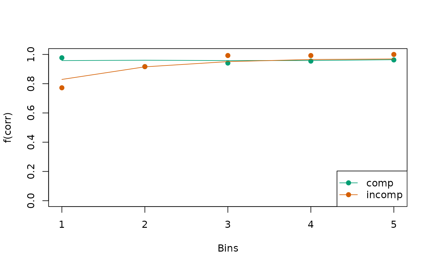

#> Aggregating across ID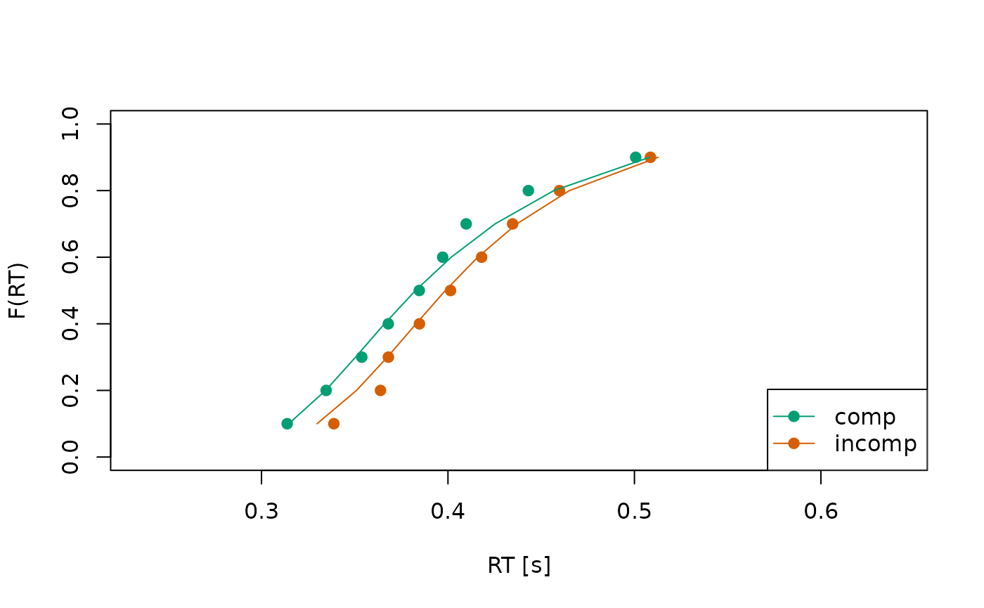

Circles indicate observed data while lines indicate the model’s predictions.

To invoke a bootstrap, where we repeatedly resample individuals to derive an uncertainty interval around both the observed and predicted data, we can specify the argument in combination with the argument . This helps us to judge if small misfits between the observed data and the model predictions are just related to sampling noise, or whether they reflect systematic misfits that are apparent across individuals.³:

check_fit <- calc_stats(
  object = all_fits,
  type = c("cafs", "quantiles"),
  level = "group",
  resample = TRUE
)
plot(check_fit)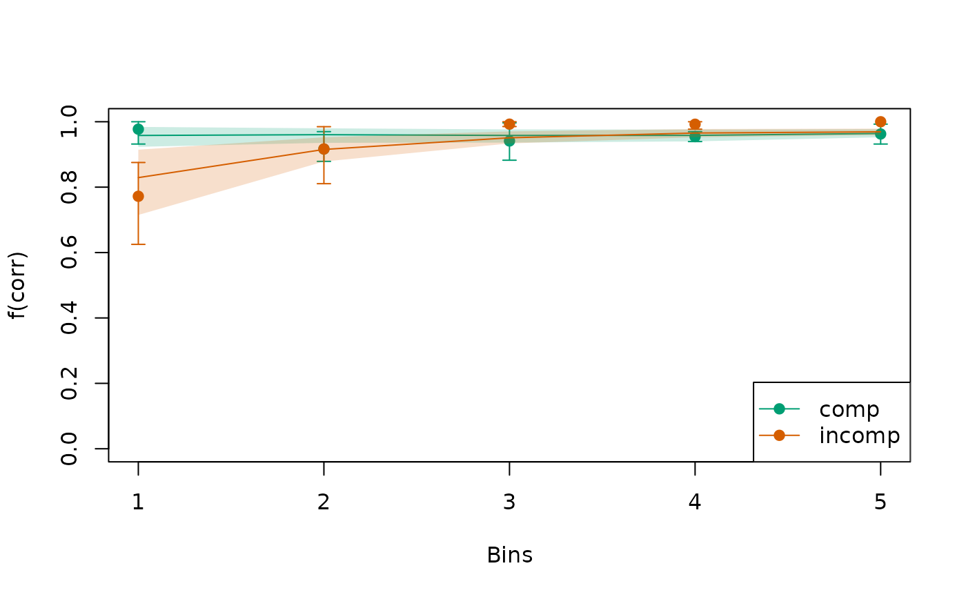

Extracting Parameter Estimates and Fit Statistics

Extracting the parameter estimates can be done via the coef() method, which work with the objects returned by estimate_dm().

all_coefs <- coef(all_fits)
print(all_coefs)
#> Object Type: coefs_dm
#> 
#>   ID   muc     b non_dec sd_non_dec   tau     A  alpha
#> 1  1 4.288 0.409   0.315      0.035 0.023 0.090  9.046
#> 2  2 4.260 0.378   0.305      0.032 0.061 0.018  4.321
#> 3  3 5.177 0.404   0.307      0.018 0.012 0.067 15.440
#> 4  4 2.878 0.534   0.304      0.035 0.043 0.096  2.832
#> 
#> (access the data.frame's columns/rows as usual)

We can even make a quick visualization of the respective distributions using the hist() method.

hist(all_coefs, bundle_plots = FALSE)

After fitting a model, we often want to quantify its fit—and maybe compare the quantiative fit between several candidate models. To this end, we can request several relative and absolute fit measures, using calc_stats() and the argument type = "fit_stats".

calc_stats(all_fits, type = "fit_stats")
#> Type of Statistic: fit_stats
#> 
#>   ID Log_Like Neg_Log_Like       AIC      BIC RMSE_s RMSE_ms
#> 1  1  417.937     -417.937  -821.874 -795.154  0.029  29.078
#> 2  2  382.680     -382.680  -751.360 -724.640  0.043  42.654
#> 3  3  512.195     -512.195 -1010.389 -983.670  0.014  13.963
#> 4  4  172.065     -172.065  -330.129 -303.493  0.040  40.187
#> 
#> (access the data.frame's columns/rows as usual)

The first few columns provide the (negative) log-likelihood, and the Akaike and Bayesian Information Criterion. The last two columns provide the RMSE statistic (in the unit of seconds and milliseconds).

A neat summary of the model, the optimization routine, the data, and the parameter estimates can be obtained via the summary() method.

summary(all_fits)
#> Fit approach: separately - classical
#> Fitted model type: dmc_dm, drift_dm
#> Optimizer: Nelder-Mead 
#> Convergence: Failed for 1 participant 
#> N Individuals: 4 
#> Average Trial Numbers:
#>  167 trials comp; 168 trials incomp
#> Cost Function: neg_log_like
#> 
#> Parameter Summary: comp 
#>           muc     b non_dec sd_non_dec   tau a     A alpha peak_l
#> mean    4.151 0.431   0.308      0.030 0.035 2 0.068 7.910  0.035
#> std_err 0.475 0.035   0.002      0.004 0.011 0 0.018 2.838  0.011
#> 
#> Parameter Summary: incomp 
#>           muc     b non_dec sd_non_dec   tau a      A alpha peak_l
#> mean    4.151 0.431   0.308      0.030 0.035 2 -0.068 7.910  0.035
#> std_err 0.475 0.035   0.002      0.004 0.011 0  0.018 2.838  0.011
#> 
#> -------
#> Deriving PDFS:
#>   solver: kfe
#>   values: sigma=1, t_max=3, dt=0.0075, dx=0.02, nt=400, nx=100

Experimental: Perform Bayesian Parameter Estimation

Starting with dRiftDM v.0.3.0, there is also the option to perform Bayesian parameter estimation using DE-MCMC. Yet, this is currently at an experimental stage, and the returned mcmc_dm object type is not yet fully integrated within the remaining dRiftDM framework.

We can request Bayesian parameter estimation using the argument approach = "sep_b" or approach = "hier_b". In the former case, the model is fitted separately per participant, in the latter case, the model is fitted hierarchically.

The prior distributions can be parameterized using the arguments lower, upper, means, sds, shapes, and rates (see the documentation of estimate_dm())

# DMC without variability in the non-decision time;
# makes it a bit easier to estimate, although it is still
# difficult, because trial numbers are low in the sample data set :)
ddm <- dmc_dm(var_non_dec = FALSE)

# lower and upper boundary for the prior distributions
l_u <- get_lower_upper(ddm)
mcmc_list <- estimate_dm(
  drift_dm_obj = ddm,
  obs_data = data,
  approach = "sep_b",
  lower = l_u$lower,
  upper = l_u$upper,
  verbose = 2,
  n_chains = 40,
  n_cores = 1, # increase to parallelize
  burn_in = 150, # for the demo, usually a bit higher
  samples = 150, # for the demo, usually a bit higher
  seed = 1
)

This returns a list of mcmc_dm objects, one for each individual.

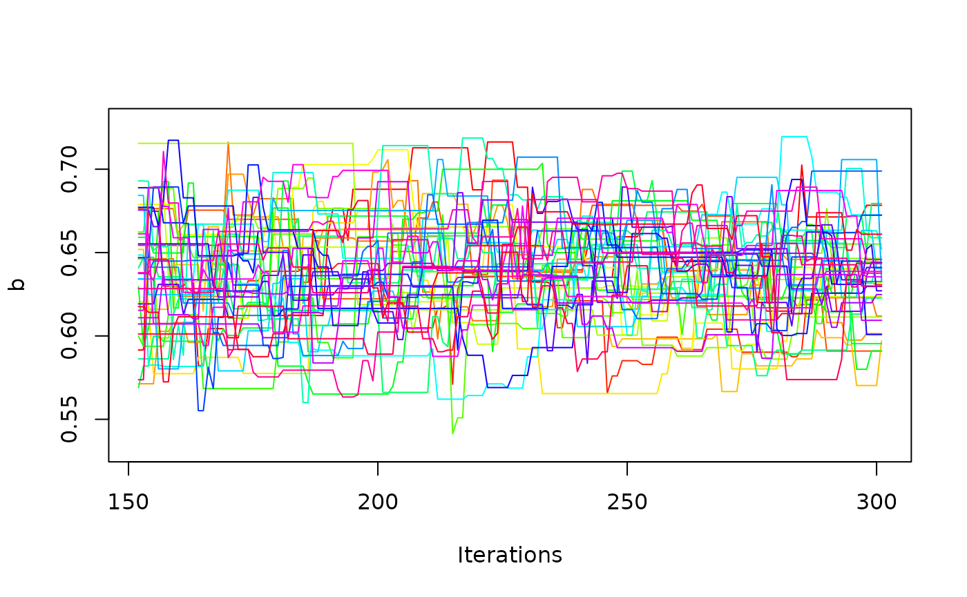
one_mcmc <- mcmc_list[[1]]
one_mcmc
#> Sampler: DE-MCMC 
#> Hierarchical: FALSE 
#> No. Parameters: 6 
#> No. Chains: 40 
#> Iterations Per Chain: 150
coef(one_mcmc)
#>        muc          b    non_dec        tau          A      alpha 
#> 4.44719079 0.63874750 0.26239573 0.06165401 0.08431614 6.88167399
plot(one_mcmc, bundle_plots = FALSE)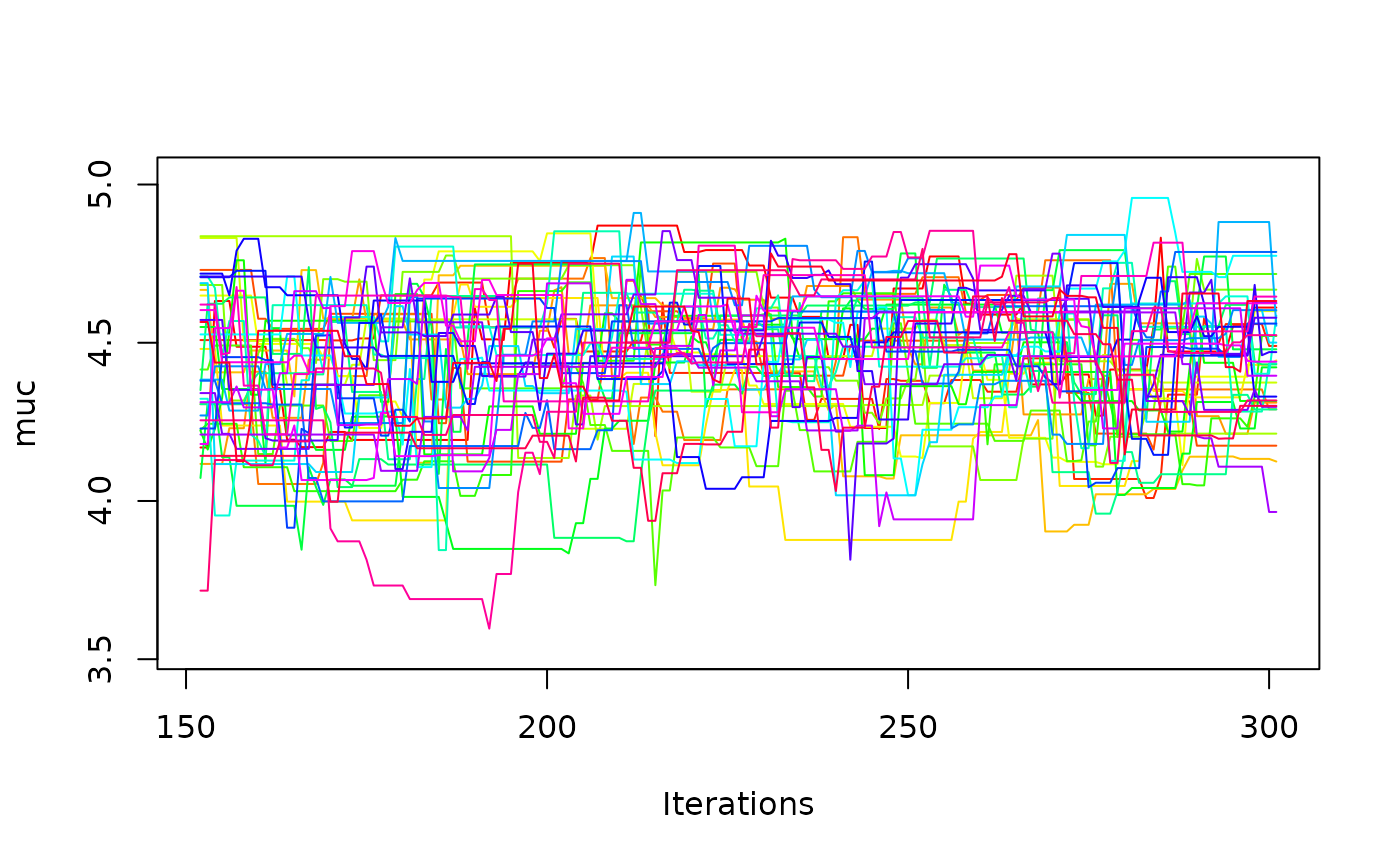

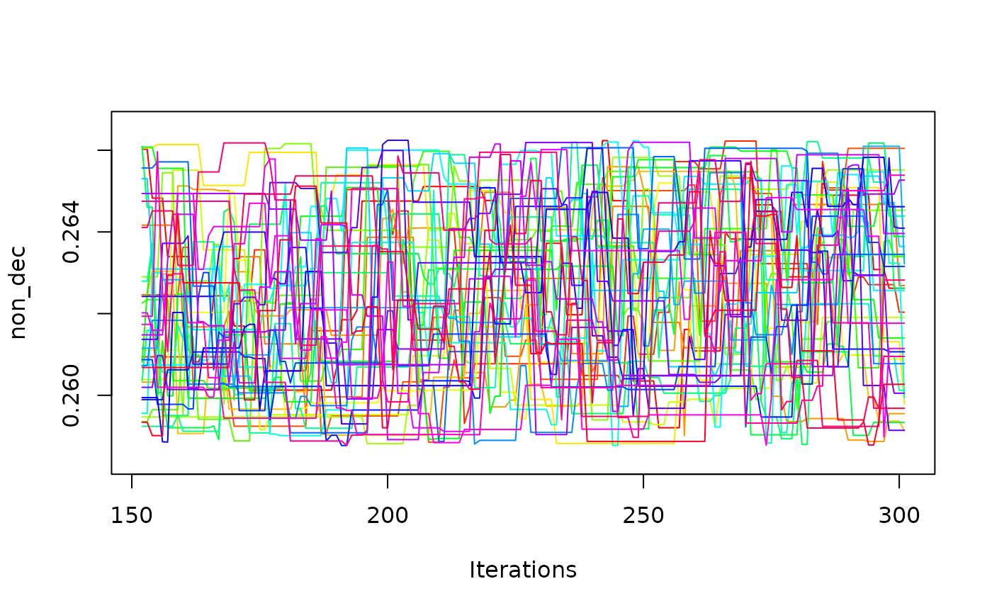
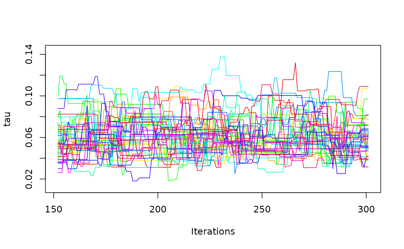
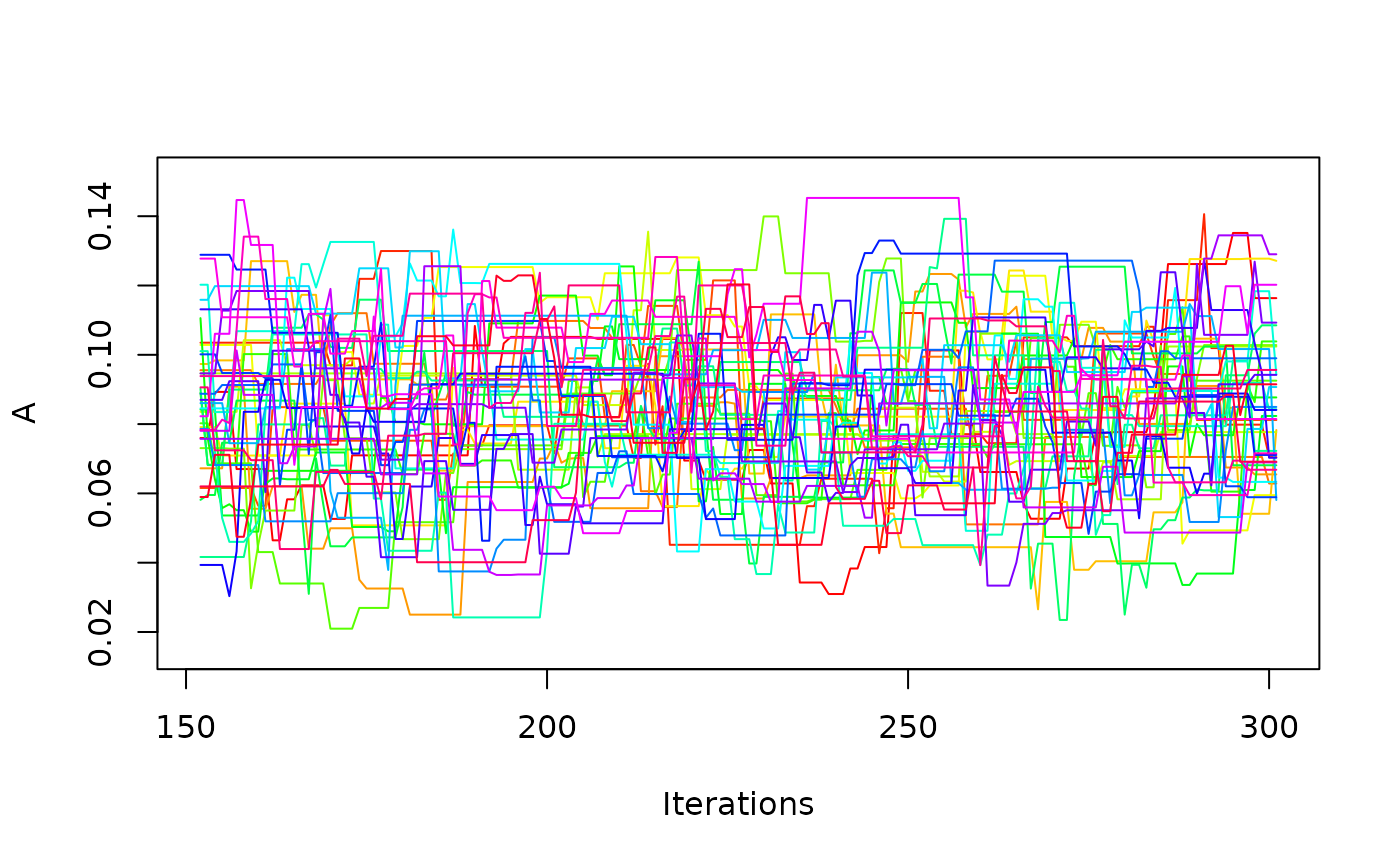
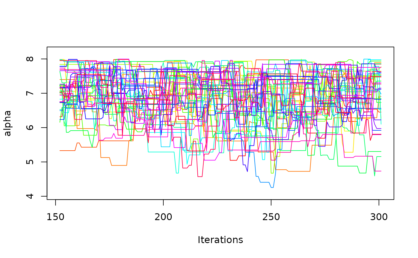
It is also possible to request hierarchical estimation.

mcmc_hier <- estimate_dm(
  drift_dm_obj = ddm,
  obs_data = data,
  approach = "hier_b",
  lower = l_u$lower,
  upper = l_u$upper,
  verbose = 2,
  n_chains = 40,
  n_cores = 1, # increase for speed-up
  burn_in = 150, # for the demo, usually way higher
  samples = 150, # for the demo, usually way higher
  seed = 1
)

Simulating Data

To simulate data based on a model, we can use the simulate_data() function. The first argument takes the model object. The second argument is a numeric (vector), defining the number of trials per condition:

ddm <- ratcliff_dm() # a model for demonstration purpose
sim_1 <- simulate_data(object = ddm, n = 200)
head(sim_1)
#>      RT Error Cond
#> 1 0.651     0 null
#> 2 0.405     0 null
#> 3 0.441     0 null
#> 4 0.426     0 null
#> 5 0.490     0 null
#> 6 0.440     0 null

This returns a single synthetic data set for one “participant”. Note that the simulated response times are rounded to three digits per default.

By specifying the argument k, we can simulate multiple synthetic data sets simultaneously. In this case, however, we must also specify lower and upper bounds to define the simulation space when drawing random parameter combinations per data set (see the simulate_data documentation for more details):

sim_2 <- simulate_data(
  object = ddm, n = 200, k = 2,
  lower = c(muc = 1, b = .4, non_dec = .2),
  upper = c(muc = 6, b = .8, non_dec = .4)
)

This returns a list with the synthetic data sets and the corresponding parameter values:

head(sim_2$synth_data)
#>      RT Error Cond ID
#> 1 0.415     0 null  1
#> 2 0.394     0 null  1
#> 3 0.504     0 null  1
#> 4 0.435     0 null  1
#> 5 0.376     0 null  1
#> 6 0.389     0 null  1
head(sim_2$prms)
#>   ID      muc         b   non_dec
#> 1  1 5.244792 0.7871501 0.3069412
#> 2  2 1.532809 0.6139069 0.2390046

The returned data sets are in a format that can be passed directly to estimate_model_ids(), making parameter recovery exercises very easy.

Remark: Stripping Away “Unnecesary” Attributes and Class Labels

Many functions in dRiftDM return matrices or data.frames. Often these returned objects are S3 objects with a custom class label. In principle, this is great because it allows you to reuse generic functions like plot(), print(), or summary() as we saw above.

However, sometimes this also hides the true structure of the underlying data type. Therefore, we provide the unpack_obj() function, which allows you to strip away unnecessary attributes and class labels. This can be useful, for example, if you want to create your own plot or wrangle the data into a particular format.

ddm <- dmc_dm()
traces <- simulate_traces(ddm, k = 2)
# although this object is essentially a list of matrices, the class label ...
class(traces)
#> [1] "traces_dm_list"
print(traces) # ... leads to nicely formatted output; but hides the underlying structure
#> Class(es): traces_dm_list
#> 
#> Time space:
#> 0.000, 0.007, 0.015, 0.022 ... 3.000 
#> 
#> Condition: comp 
#> ~>  0.000,  0.016,  0.136,  0.164 ...  0.646 
#> ~>  0.000,  0.078,  0.387,  0.372 ...  0.656 
#> 
#> Condition: incomp 
#> ~>  0.000, -0.203, -0.190, -0.037 ...  0.646 
#> ~>  0.000, -0.027, -0.090, -0.085 ...  0.614

raw <- unpack_obj(traces) # provides the plain list of matrices
head(t(raw$comp))
#>            [,1]       [,2]
#> [1,] 0.00000000 0.00000000
#> [2,] 0.01610337 0.07827198
#> [3,] 0.13579594 0.38695708
#> [4,] 0.16438534 0.37209682
#> [5,] 0.10007293 0.45559657
#> [6,] 0.18377312 0.42206136

Janczyk, Markus, Ian Grant Mackenzie, and Valentin Koob. 2024. “A Comment on the Revised Diffusion Model for Conflict Tasks (RDMC).” Psychonomic Bulletin & Review, 1–15.

Ratcliff, Roger. 1978. “A Theory of Memory Retrieval.” Psychological Review 85 (2): 59–108. https://doi.org/10.1037/0033-295X.85.2.59.

Richter, Thomas, Rolf Ulrich, and Markus Janczyk. 2023. “Diffusion Models with Time-Dependent Parameters: An Analysis of Computational Effort and Accuracy of Different Numerical Methods.” Journal of Mathematical Psychology 114: 102756. https://doi.org/10.1016/j.jmp.2023.102756.

Ulrich, Rolf, Hannes Schröter, Hartmut Leuthold, and Teresa Birngruber. 2015. “Automatic and Controlled Stimulus Processing in Conflict Tasks: Superimposed Diffusion Processes and Delta Functions.” Cognitive Psychology 78: 148–74. https://doi.org/10.1016/j.cogpsych.2015.02.005.

White, Corey N, Roger Ratcliff, and Jeffrey J Starns. 2011. “Diffusion Models of the Flanker Task: Discrete Versus Gradual Attentional Selection.” Cognitive Psychology 63 (4): 210–38. https://doi.org/10.1016/j.cogpsych.2011.08.001.